An open-source library for time series forecasting released by Meta (formerly Facebook).
For installation instructions in Python, refer to Installation in Python.
Generally, you can install it by running pip install prophet
.
Taylor, Sean J., and Benjamin Letham. “Forecasting at scale.” The American Statistician 72.1 (2018): 37-45.
import numpy as np
import pandas as pd
import seaborn as sns
import matplotlib.pyplot as plt
import japanize_matplotlib
from prophet import Prophet
Data Used for the Experiment #
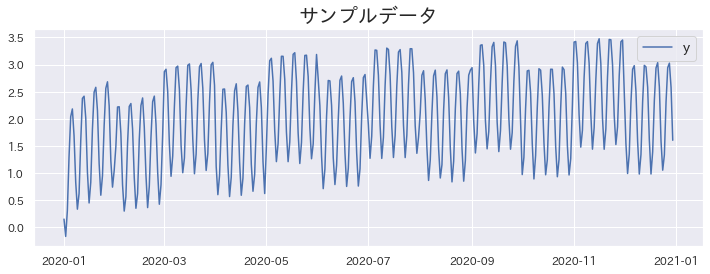
We will use one year of data. Even-numbered months tend to show a decrease in values. Additionally, the data exhibits periodic patterns on a weekly basis.
The data covers the period from 2020/1/1 to 2020/12/31.
date = pd.date_range("2020-01-01", periods=365, freq="D")
# Target variable for forecasting
y = [
np.cos(di.weekday())
+ di.month % 2 / 2
+ np.log(i + 1) / 3.0
+ np.random.rand() / 10
for i, di in enumerate(date)
]
# Trend component
x = [18627 + i - 364 for i in range(365)]
trend_y = [np.log(i + 1) / 3.0 for i, di in enumerate(date)]
weekly_y = [np.cos(di.weekday()) for i, di in enumerate(date)]
seasonal_y = [di.month % 2 / 2 for i, di in enumerate(date)]
noise_y = [np.random.rand() / 10 for i in range(365)]
df = pd.DataFrame({"ds": date, "y": y})
df.index = date
# Data used in the experiment
plt.title("Sample Data")
sns.lineplot(data=df)
plt.show()
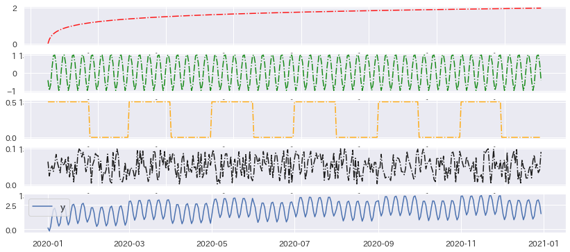
Components of Time Series Data #
The term “time series data” encompasses various types of data.
Here, we focus on the following type of data:
- Data consisting only of timestamps and numerical values.
- Timestamps are evenly spaced with no missing values.
plt.figure(figsize=(14, 6))
plt.title("Decomposing y into its components")
plt.subplot(511)
plt.plot(x, trend_y, "-.", color="red", label="Trend", alpha=0.9)
plt.subplot(512)
plt.plot(x, weekly_y, "-.", color="green", label="Periodic Fluctuation (Weekly)", alpha=0.9)
plt.subplot(513)
plt.plot(x, seasonal_y, "-.", color="orange", label="Periodic Fluctuation (Monthly)", alpha=0.9)
plt.subplot(514)
plt.plot(x, noise_y, "-.", color="k", label="Noise Component")
plt.subplot(515)
sns.lineplot(data=df)
plt.show()
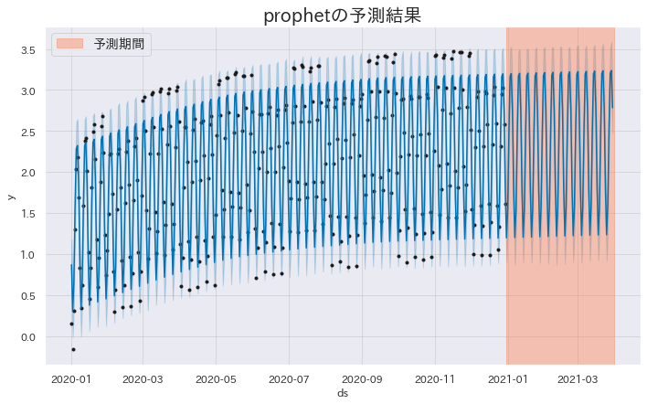
Forecasting January to March 2021 with Prophet #
Using the data from 2020/1/1 to 2020/12/31, we will forecast the next three months.
Since we only have one year of data, we set yearly_seasonality=False
.
Because the data exhibits weekly periodicity, we set daily_seasonality=True
.
def train_and_forecast_pf(
data,
periods=90,
yearly_seasonality=False,
weekly_seasonality=True,
daily_seasonality=True,
):
"""Train a Prophet model and forecast future values.
Args:
data (pandas.DataFrame): Time series data.
periods (int, optional): Length of the forecast period. Defaults to 90.
yearly_seasonality (bool, optional): Whether annual seasonality is present. Defaults to False.
weekly_seasonality (bool, optional): Whether weekly seasonality is present. Defaults to True.
daily_seasonality (bool, optional): Whether daily seasonality is present. Defaults to True.
Returns:
_type_: Forecast model, forecast results.
"""
assert "ds" in data.columns and "y" in data.columns, "The input data must contain 'ds' and 'y' columns."
# Train the model
m = Prophet(
yearly_seasonality=yearly_seasonality,
weekly_seasonality=weekly_seasonality,
daily_seasonality=daily_seasonality,
)
m.fit(df)
# Make future predictions
future = m.make_future_dataframe(periods=periods)
forecast = m.predict(future)
return m, forecast
# Check the forecast results
periods = 90
m, forecast = train_and_forecast_pf(
df,
periods=periods,
yearly_seasonality=False,
weekly_seasonality=True,
daily_seasonality=True,
)
fig = m.plot(forecast)
plt.title("Prophet Forecast Results")
plt.axvspan(18627, 18627 + periods, color="coral", alpha=0.4, label="Forecast Period")
plt.legend()
plt.show()
Initial log joint probability = -32.1541
Iter log prob ||dx|| ||grad|| alpha alpha0 # evals Notes
99 772.276 5.98161e-05 56.7832 1 1 135
Iter log prob ||dx|| ||grad|| alpha alpha0 # evals Notes
131 772.59 0.00128893 157.592 1.465e-05 0.001 217 LS failed, Hessian reset
181 772.678 3.78737e-05 49.0389 6.852e-07 0.001 326 LS failed, Hessian reset
199 772.681 1.42622e-06 43.2231 0.6929 0.6929 350
Iter log prob ||dx|| ||grad|| alpha alpha0 # evals Notes
230 772.681 6.80165e-06 56.0478 7.185e-08 0.001 432 LS failed, Hessian reset
245 772.681 4.06967e-08 48.5475 0.1802 0.8285 454
Optimization terminated normally:
Convergence detected: relative gradient magnitude is below tolerance
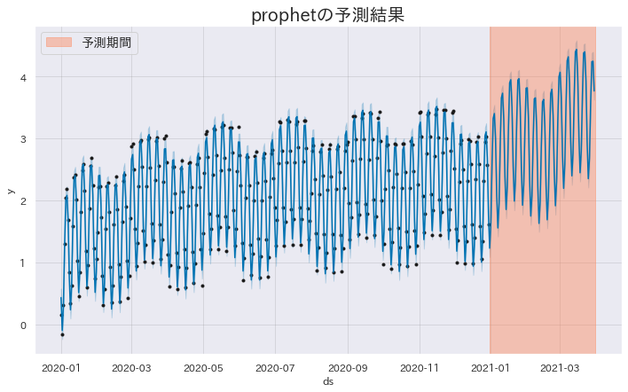
Impact of Specifying Seasonality #
In the example below, we deliberately specify that there is annual seasonality (yearly_seasonality=True). Due to the term introduced to capture the yearly cycle, the forecast for 2022 shows a somewhat unnatural increase.
# Check the forecast results
periods = 90
m, forecast = train_and_forecast_pf(
df,
periods=periods,
yearly_seasonality=False,
weekly_seasonality=True,
daily_seasonality=True,
)
fig = m.plot(forecast)
plt.title("Prophet Forecast Results")
plt.axvspan(18627, 18627 + periods, color="coral", alpha=0.4, label="Forecast Period")
plt.legend()
plt.show()
Initial log joint probability = -32.1541
Iter log prob ||dx|| ||grad|| alpha alpha0 # evals Notes
99 1076.54 0.000445309 68.8033 1 1 133
Iter log prob ||dx|| ||grad|| alpha alpha0 # evals Notes
199 1078.13 0.000151685 92.7241 1 1 256
Iter log prob ||dx|| ||grad|| alpha alpha0 # evals Notes
246 1078.14 1.78997e-06 84.0649 1.52e-08 0.001 353 LS failed, Hessian reset
261 1078.14 3.82403e-08 101.692 0.2973 1 372
Optimization terminated normally:
Convergence detected: relative gradient magnitude is below tolerance