<p>Time-series data changes its waveform over time, but it may increase or decrease over time. Such gradual, non-periodic changes are sometimes referred to as trends.
Data with a trend changes the mean, variance, and other statistics of the data over time, and as a result is more difficult to predict.
On this page, we will try to remove the trend component from time series data using python.</p>
1
2
3
4
| import pandas as pd
import matplotlib.pyplot as plt
import numpy as np
import seaborn as sns
|
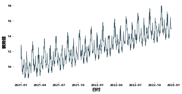
Generate sample data
#
 1
 2
 3
 4
 5
 6
 7
 8
 9
10
11
12
13
14
15
16
17
18
| date_list = pd.date_range("2021-01-01", periods=720, freq="D")
value_list = [
10
+ np.cos(np.pi * i / 28.0) * (i % 3 > 0)
+ np.cos(np.pi * i / 14.0) * (i % 5 > 0)
+ np.cos(np.pi * i / 7.0)
+ (i / 10) ** 1.1 / 20
for i, di in enumerate(date_list)
]
df = pd.DataFrame(
{
"日付": date_list,
"y": value_list,
}
)
df.head(10)
|
| 日付 | y |
|---|
| 0 | 2021-01-01 | 11.000000 |
|---|
| 1 | 2021-01-02 | 12.873581 |
|---|
| 2 | 2021-01-03 | 12.507900 |
|---|
| 3 | 2021-01-04 | 11.017651 |
|---|
| 4 | 2021-01-05 | 11.320187 |
|---|
| 5 | 2021-01-06 | 10.246560 |
|---|
| 6 | 2021-01-07 | 9.350058 |
|---|
| 7 | 2021-01-08 | 9.740880 |
|---|
| 8 | 2021-01-09 | 9.539117 |
|---|
| 9 | 2021-01-10 | 8.987155 |
|---|
1
2
| plt.figure(figsize=(10, 5))
sns.lineplot(x=df["日付"], y=df["y"])
|
Forecast Time Series Data with XGBoost
#
1
2
3
4
5
6
7
8
9
10
11
12
13
14
15
16
17
18
19
20
21
22
23
24
25
26
27
28
29
30
| df["曜日"] = df["日付"].dt.weekday
df["年初からの日数%14"] = df["日付"].dt.dayofyear % 14
df["年初からの日数%28"] = df["日付"].dt.dayofyear % 28
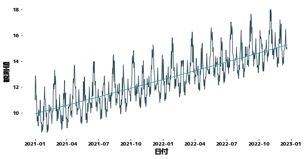
def get_trend(timeseries, deg=3, trainN=0):
"""Create a trend line for time-series data
Args:
timeseries(pd.Series) : Time series data
deg(int) : Degree of polynomial
trainN(int): Number of data used to estimate the coefficients of the polynomial
Returns:
pd.Series: Time series data corresponding to trends
"""
if trainN == 0:
trainN = len(timeseries)
x = list(range(len(timeseries)))
y = timeseries.values
coef = np.polyfit(x[:trainN], y[:trainN], deg)
trend = np.poly1d(coef)(x)
return pd.Series(data=trend, index=timeseries.index)
trainN = 500
df["Trend"] = get_trend(df["y"], trainN=trainN, deg=2)
plt.figure(figsize=(10, 5))
sns.lineplot(x=df["日付"], y=df["y"])
sns.lineplot(x=df["日付"], y=df["Trend"])
|
1
2
3
4
5
6
| X = df[["曜日", "年初からの日数%14", "年初からの日数%28"]]
y = df["y"]
trainX, trainy = X[:trainN], y[:trainN]
testX, testy = X[trainN:], y[trainN:]
trend_train, trend_test = df["Trend"][:trainN], df["Trend"][trainN:]
|
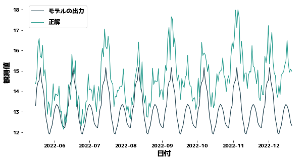
Forecasting without considering trends
#
XGBoost does not know that data changes slowly between training and test data.
Therefore, the more you predict the future, the more your predictions will be off down the road.
For XGBoost to forecast well, the y distribution of the training and test data must be close.
 1
 2
 3
 4
 5
 6
 7
 8
 9
10
11
12
| import xgboost as xgb
from sklearn.metrics import mean_squared_error
regressor = xgb.XGBRegressor(max_depth=5).fit(trainX, trainy)
prediction = regressor.predict(testX)
plt.figure(figsize=(10, 5))
sns.lineplot(x=df["日付"][trainN:], y=prediction)
sns.lineplot(x=df["日付"][trainN:], y=testy)
plt.legend(["モデルの出力", "正解"], bbox_to_anchor=(0.0, 0.78, 0.28, 0.102))
print(f"MSE = {mean_squared_error(testy, prediction)}")
|
MSE = 2.815118389938834
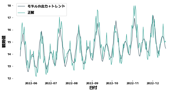
Forecasting with the trend taken into account
#
We first remove the portion corresponding to the trend from the observed values and then predict the values without the trend.
The XGBoost prediction is then added to the XGBoost prediction to obtain the final prediction.
 1
 2
 3
 4
 5
 6
 7
 8
 9
10
| regressor = xgb.XGBRegressor(max_depth=5).fit(trainX, trainy - trend_train)
prediction = regressor.predict(testX)
prediction = [pred_i + trend_i for pred_i, trend_i in zip(prediction, trend_test)]
plt.figure(figsize=(10, 5))
sns.lineplot(x=df["日付"][trainN:], y=prediction)
sns.lineplot(x=df["日付"][trainN:], y=testy)
plt.legend(["モデルの出力+Trend", "正解"], bbox_to_anchor=(0.0, 0.78, 0.28, 0.102))
print(f"MSE = {mean_squared_error(testy, prediction)}")
|
MSE = 0.46014173311011325