5.10.3
Trend & Periodicity
<p>Time-series data are sometimes considered to be composed of seasonality, trend components, and residuals, and there are times when we want to decompose time-series data into these three components.
STL decomposition decomposes data into seasonality, trend components, and residuals based on the specified period length. This method is effective when the length of the period of the seasonal component (waves that occur repeatedly) is constant and the length of the period is known in advance.</p>
1
2
3
4
5
| import matplotlib.pyplot as plt
import numpy as np
from statsmodels.tsa.seasonal import seasonal_decompose
from statsmodels.tsa.seasonal import STL
|
Sample data created
#
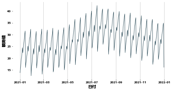
The data is a combination of several periodic values, and the trend changes in a segmented manner. Noise is also added by np.random.rand().
 1
 2
 3
 4
 5
 6
 7
 8
 9
10
11
12
13
14
15
16
17
18
19
20
| date_list = pd.date_range("2021-01-01", periods=365, freq="D")
value_list = [
10
+ i % 14
+ np.log(1 + i % 28 + np.random.rand())
+ np.sqrt(1 + i % 7 + np.random.rand()) * 2
+ (((i - 100) / 10)) * (i > 100)
- ((i - 200) / 7) * (i > 200)
+ np.random.rand()
for i, di in enumerate(date_list)
]
df = pd.DataFrame(
{
"日付": date_list,
"観測値": value_list,
}
)
df.head(10)
|
| 日付 | 観測値 |
|---|
| 0 | 2021-01-01 | 13.874478 |
|---|
| 1 | 2021-01-02 | 15.337944 |
|---|
| 2 | 2021-01-03 | 17.166133 |
|---|
| 3 | 2021-01-04 | 19.561274 |
|---|
| 4 | 2021-01-05 | 20.426502 |
|---|
| 5 | 2021-01-06 | 22.127725 |
|---|
| 6 | 2021-01-07 | 24.484329 |
|---|
| 7 | 2021-01-08 | 22.313675 |
|---|
| 8 | 2021-01-09 | 23.716303 |
|---|
| 9 | 2021-01-10 | 25.861587 |
|---|
1
2
3
4
| plt.figure(figsize=(10, 5))
sns.lineplot(x=df["日付"], y=df["観測値"])
plt.grid(axis="x")
plt.show()
|
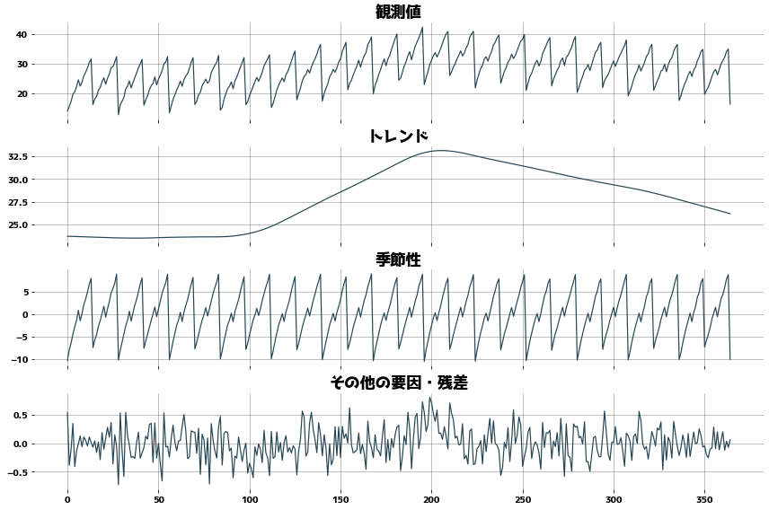
Decompose into trend, periodicity, and residuals
#
Time series data using statsmodels.tsa.seasonal.STL
- Trend (.trend)
- Seasonal/periodic(.seasonal)
- Residual(.resid)
(In the following code, dr means DecomposeResult.
Cleveland, Robert B., et al. “STL: A seasonal-trend decomposition.” J. Off. Stat 6.1 (1990): 3-73. (pdf)
1
2
3
| period = 28
stl = STL(df["観測値"], period=period)
dr = stl.fit()
|
 1
 2
 3
 4
 5
 6
 7
 8
 9
10
11
12
13
14
15
16
17
18
19
20
| _, axes = plt.subplots(figsize=(12, 8), ncols=1, nrows=4, sharex=True)
axes[0].set_title("観測値")
axes[0].plot(dr.observed)
axes[0].grid()
axes[1].set_title("トレンド")
axes[1].plot(dr.trend)
axes[1].grid()
axes[2].set_title("季節性")
axes[2].plot(dr.seasonal)
axes[2].grid()
axes[3].set_title("その他の要因・残差")
axes[3].plot(dr.resid)
axes[3].grid()
plt.tight_layout()
plt.show()
|
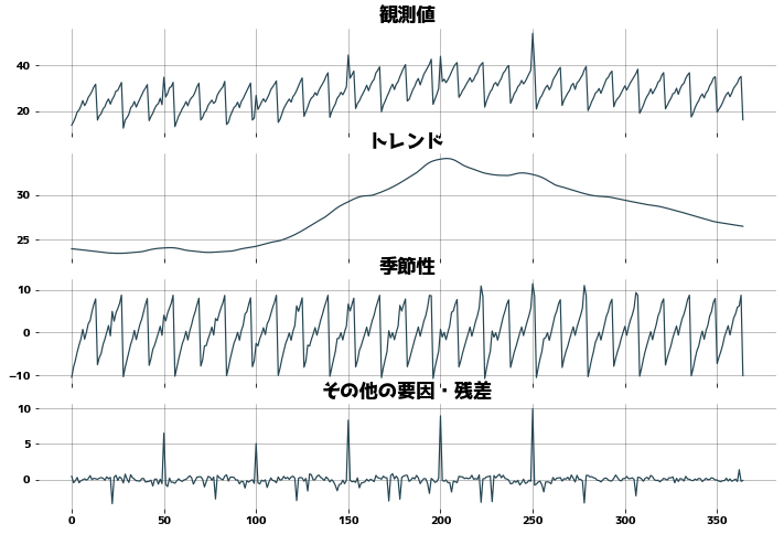
Check for resistance to outliers
#
 1
 2
 3
 4
 5
 6
 7
 8
 9
10
11
12
13
14
15
16
17
18
19
20
21
22
23
24
25
26
27
28
29
| def check_outlier():
period = 28
df_outlier = df["観測値"].copy()
for i in range(1, 6):
df_outlier[i * 50] = df_outlier[i * 50] * 1.4
stl = STL(df_outlier, period=period, trend=31)
dr_outlier = stl.fit()
_, axes = plt.subplots(figsize=(12, 8), ncols=1, nrows=4, sharex=True)
axes[0].set_title("観測値")
axes[0].plot(dr_outlier.observed)
axes[0].grid()
axes[1].set_title("トレンド")
axes[1].plot(dr_outlier.trend)
axes[1].grid()
axes[2].set_title("季節性")
axes[2].plot(dr_outlier.seasonal)
axes[2].grid()
axes[3].set_title("その他の要因・残差")
axes[3].plot(dr_outlier.resid)
axes[3].grid()
check_outlier()
|
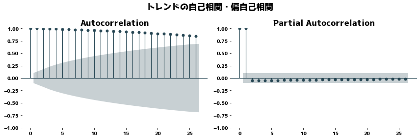
If the trend is correctly extracted, the trend should not contain a cyclical component and the PACF (Partial Autocorrelation) should be close to zero.
 1
 2
 3
 4
 5
 6
 7
 8
 9
10
11
12
13
14
15
| from statsmodels.graphics.tsaplots import plot_acf, plot_pacf
_, axes = plt.subplots(nrows=1, ncols=2, figsize=(12, 4))
plt.suptitle("トレンドの自己相関・偏自己相関")
plot_acf(dr.trend.dropna(), ax=axes[0])
plot_pacf(dr.trend.dropna(), method="ywm", ax=axes[1])
plt.tight_layout()
plt.show()
_, axes = plt.subplots(nrows=1, ncols=2, figsize=(12, 4))
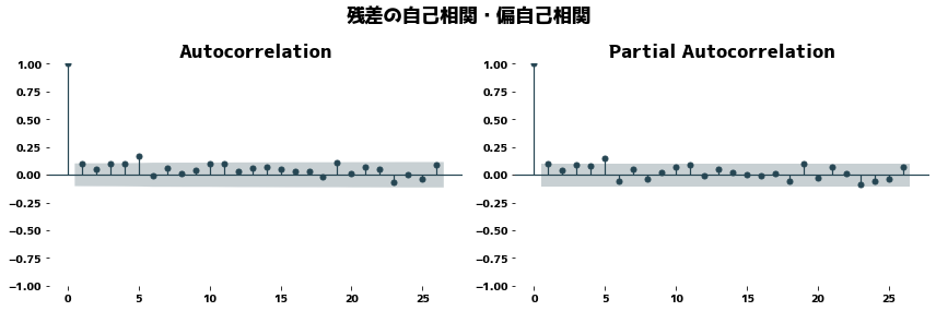
plt.suptitle("残差の自己相関・偏自己相関")
plot_acf(dr.resid.dropna(), ax=axes[0])
plot_pacf(dr.resid.dropna(), method="ywm", ax=axes[1])
plt.tight_layout()
plt.show()
|
Portmanteau test
#
1
2
3
| from statsmodels.stats.diagnostic import acorr_ljungbox
acorr_ljungbox(dr.resid.dropna(), lags=int(np.log(df.shape[0])))
|
| lb_stat | lb_pvalue |
|---|
| 1 | 3.962297 | 0.046530 |
|---|
| 2 | 4.823514 | 0.089658 |
|---|
| 3 | 8.456753 | 0.037457 |
|---|
| 4 | 12.092893 | 0.016674 |
|---|
| 5 | 23.134467 | 0.000318 |
|---|