5.10.4
Box-Cox transformation
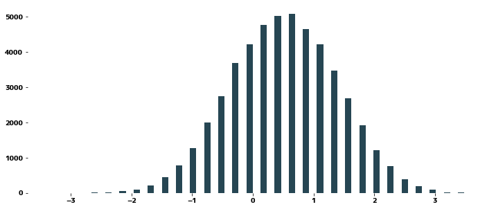
<p>Pre-processing may be required to analyze time series data using a model. This is because time series models are not capable of analyzing any data, and often make assumptions such as "variance is always constant" or "follows a normal distribution. Here we will use the Box-Cox transformation to transform slightly biased data into a near normal distribution and see how this affects the output of the model (distribution of errors between correct and predicted values).</p>
1
2
| import matplotlib.pyplot as plt
import numpy as np
|
 1
 2
 3
 4
 5
 6
 7
 8
 9
10
11
12
| from scipy import stats
import numpy as np
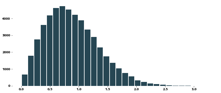
plt.figure(figsize=(12, 5))
data_wb = np.random.weibull(2.0, size=50000)
plt.hist(data_wb, bins=30, rwidth=0.9)
plt.show()
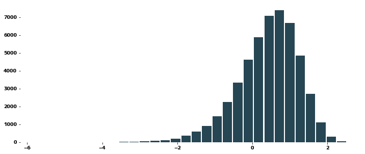
plt.figure(figsize=(12, 5))
data_lg = stats.loggamma.rvs(2.0, size=50000)
plt.hist(data_lg, bins=30, rwidth=0.9)
plt.show()
|
1
2
3
4
5
| from scipy.stats import boxcox
plt.figure(figsize=(12, 5))
plt.hist(boxcox(data_wb), bins=30, rwidth=0.9)
plt.show()
|
1
2
3
4
5
6
| try:
plt.figure(figsize=(12, 5))
plt.hist(boxcox(data_lg), bins=30, rwidth=0.9)
plt.show()
except ValueError as e:
print(f"エラーの内容: ValueError {e.args}")
|
エラーの内容: ValueError ('Data must be positive.',)

<Figure size 864x360 with 0 Axes>
1
2
3
4
5
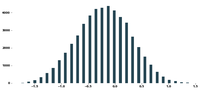
| from scipy.stats import yeojohnson
plt.figure(figsize=(12, 5))
plt.hist(yeojohnson(data_lg), bins=30, rwidth=0.9)
plt.show()
|
Fitting Ridge Regression
#
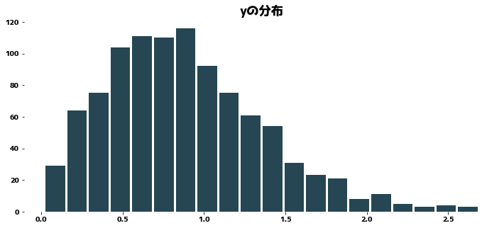
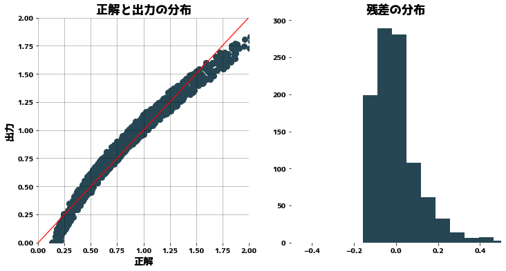
If we apply ridge regression without making the distribution of y closer to a normal distribution, we find that the distribution of the residuals is biased.
 1
 2
 3
 4
 5
 6
 7
 8
 9
10
11
12
13
| from sklearn.linear_model import Ridge
N = 1000
rng = np.random.RandomState(0)
y = np.random.weibull(2.0, size=N)
X = rng.randn(N, 5)
X[:, 0] = np.sqrt(y) + np.random.rand(N) / 10
plt.figure(figsize=(12, 5))
plt.hist(y, bins=20, rwidth=0.9)
plt.title("yの分布")
plt.show()
|
 1
 2
 3
 4
 5
 6
 7
 8
 9
10
11
12
13
14
15
16
17
18
19
| clf = Ridge(alpha=1.0)
clf.fit(X, y)
pred = clf.predict(X)
plt.figure(figsize=(12, 6))
plt.subplot(121)
plt.title("正解と出力の分布")
plt.scatter(y, pred)
plt.plot([0, 2], [0, 2], "r")
plt.xlabel("正解")
plt.ylabel("出力")
plt.xlim(0, 2)
plt.ylim(0, 2)
plt.grid()
plt.subplot(122)
plt.title("残差の分布")
plt.hist(y - pred)
plt.xlim(-0.5, 0.5)
plt.show()
|
 1
 2
 3
 4
 5
 6
 7
 8
 9
10
11
12
13
14
15
16
17
18
19
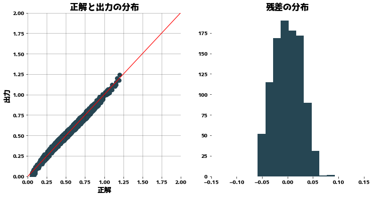
| clf = Ridge(alpha=1.0)
clf.fit(X, yeojohnson(y)[0])
pred = clf.predict(X)
plt.figure(figsize=(12, 6))
plt.subplot(121)
plt.title("正解と出力の分布")
plt.scatter(yeojohnson(y)[0], pred)
plt.plot([0, 2], [0, 2], "r")
plt.xlabel("正解")
plt.ylabel("出力")
plt.xlim(0, 2)
plt.ylim(0, 2)
plt.grid()
plt.subplot(122)
plt.title("残差の分布")
plt.hist(yeojohnson(y)[0] - pred)
plt.xlim(-0.15, 0.15)
plt.show()
|