5.13.1
Dynamic Time Warping
Summary- Dynamic Time Warping (DTW) aligns two time series while allowing for local stretching or shrinking of the time axis.
- The algorithm builds a distance matrix, computes cumulative costs with dynamic programming, and retrieves the minimal warping path.
- We implement DTW with NumPy, compare it with
fastdtw, and visualise how the optimal alignment behaves.
What is DTW?
#
DTW measures the similarity between two sequences that may vary in speed or starting phase. It aligns the sequences by finding the path with the minimum cumulative distance. Typical applications include speech recognition, activity recognition from sensors, and recommendation systems that compare temporal usage patterns.
DTW in NumPy
#
 1
 2
 3
 4
 5
 6
 7
 8
 9
10
11
12
13
14
15
16
17
18
19
20
21
22
23
24
25
26
27
28
29
30
31
32
33
| import numpy as np
def dtw_distance(
x: np.ndarray,
y: np.ndarray,
window: int | None = None,
) -> tuple[float, list[tuple[int, int]]]:
n, m = len(x), len(y)
window = max(window or max(n, m), abs(n - m))
cost = np.full((n + 1, m + 1), np.inf)
cost[0, 0] = 0.0
for i in range(1, n + 1):
for j in range(max(1, i - window), min(m + 1, i + window + 1)):
dist = abs(x[i - 1] - y[j - 1])
cost[i, j] = dist + min(cost[i - 1, j], cost[i, j - 1], cost[i - 1, j - 1])
i, j = n, m
path: list[tuple[int, int]] = []
while i > 0 and j > 0:
path.append((i - 1, j - 1))
idx = np.argmin((cost[i - 1, j], cost[i, j - 1], cost[i - 1, j - 1]))
if idx == 0:
i -= 1
elif idx == 1:
j -= 1
else:
i -= 1
j -= 1
path.reverse()
return cost[n, m], path
|
Comparing three series
#
1
2
| python --version # e.g. Python 3.13.0
pip install matplotlib fastdtw
|
 1
 2
 3
 4
 5
 6
 7
 8
 9
10
11
12
13
14
15
16
17
18
| import matplotlib.pyplot as plt
from fastdtw import fastdtw
np.random.seed(42)
t = np.arange(0, 30)
series_a = 1.2 * np.sin(t / 2.0)
series_b = 1.1 * np.sin((t + 2) / 2.1) + 0.05 * np.random.randn(len(t))
series_c = 0.8 * np.cos(t / 2.0) + 0.05 * np.random.randn(len(t))
plt.figure(figsize=(10, 3))
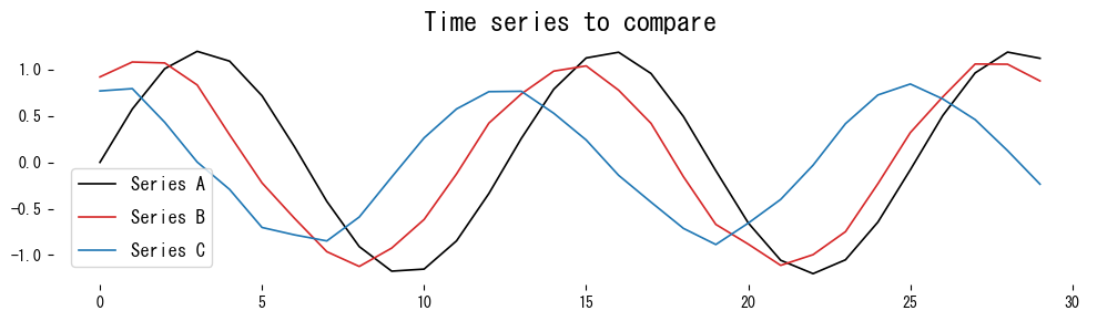
plt.plot(t, series_a, label="Series A", color="black")
plt.plot(t, series_b, label="Series B", color="tab:red")
plt.plot(t, series_c, label="Series C", color="tab:blue")
plt.title("Time series to compare")
plt.legend()
plt.tight_layout()
plt.show()
|
1
2
3
4
5
6
7
8
| dist_ab, path_ab = dtw_distance(series_a, series_b)
dist_ac, path_ac = dtw_distance(series_a, series_c)
fast_dist_ab, _ = fastdtw(series_a, series_b)
fast_dist_ac, _ = fastdtw(series_a, series_c)
print(f"DTW(A, B) = {dist_ab:.3f} / fastdtw = {fast_dist_ab:.3f}")
print(f"DTW(A, C) = {dist_ac:.3f} / fastdtw = {fast_dist_ac:.3f}")
|
Series B has a similar shape to Series A, so both DTW and fastdtw report a small distance. Series C differs in shape and therefore yields a larger distance.
Visualising the warping path
#
 1
 2
 3
 4
 5
 6
 7
 8
 9
10
11
12
13
14
15
16
17
18
19
20
21
22
23
24
25
26
27
28
| def plot_warping(a: np.ndarray, b: np.ndarray, path: list[tuple[int, int]]) -> None:
fig, axes = plt.subplots(
1,
2,
figsize=(12, 4),
gridspec_kw={"width_ratios": [1, 1.2]},
)
axes[0].plot(a, label="Series A", color="black")
axes[0].plot(b, label="Series B", color="tab:red")
axes[0].set_title("Time series")
axes[0].legend()
axes[1].imshow(
np.abs(np.subtract.outer(a, b)),
origin="lower",
interpolation="nearest",
cmap="viridis",
)
path_arr = np.array(path)
axes[1].plot(path_arr[:, 1], path_arr[:, 0], color="white", linewidth=2)
axes[1].set_title("Cumulative cost and warping path")
axes[1].set_xlabel("Series B index")
axes[1].set_ylabel("Series A index")
plt.tight_layout()
plt.show()
plot_warping(series_a, series_b, path_ab)
|
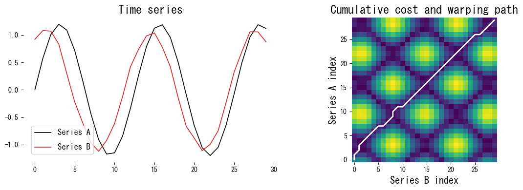
The white path reveals how the algorithm stretches Series A and Series B so that peaks and valleys align even when they are shifted in time.
Takeaways
#
- DTW aligns sequences with varying tempo by minimising cumulative distance along a warping path.
- Dynamic programming computes the optimal path; window constraints or
fastdtw can speed things up. - NumPy is sufficient for a basic implementation, and the visualisation helps debug how DTW behaves on real data.