5.13.3
tsfresh
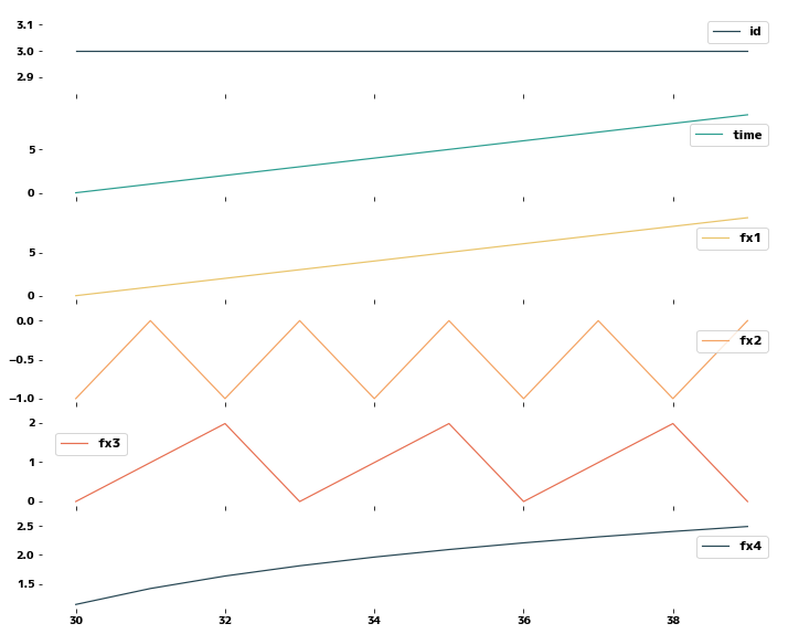
<p>When working with time series data, various features can be calculated based on timestamps and numerical values. This page demonstrates how to calculate features from time series data using tsfresh. Additionally, the accompanying video explains the perspectives from which features can be created.</p>
tsfresh #
Refer to the Overview on extracted features to see what features are generated.
| |
| id | time | fx1 | fx2 | fx3 | fx4 | |
|---|---|---|---|---|---|---|
| 0 | 0 | 0 | 0.099833 | 0.995004 | 0.100335 | -2.302585 |
| 1 | 0 | 1 | 1.099833 | 1.995004 | 1.100335 | 0.095310 |
| 2 | 0 | 2 | 2.099833 | 0.995004 | 2.100335 | 0.741937 |
| 3 | 0 | 3 | 3.099833 | 1.995004 | 0.100335 | 1.131402 |
| 4 | 0 | 4 | 4.099833 | 0.995004 | 1.100335 | 1.410987 |
| |
Calculating Features #
You can calculate all features at once using the extract_features function. Additionally, you can perform feature selection using functions available under tsfresh.feature_selection.
| |
Feature Extraction: 100%|█
| fx1__variance_larger_than_standard_deviation | fx1__has_duplicate_max | fx1__has_duplicate_min | fx1__has_duplicate | fx1__sum_values | fx1__abs_energy | fx1__mean_abs_change | fx1__mean_change | fx1__mean_second_derivative_central | fx1__median | ... | fx4__permutation_entropy__dimension_6__tau_1 | fx4__permutation_entropy__dimension_7__tau_1 | fx4__query_similarity_count__query_None__threshold_0.0 | fx4__matrix_profile__feature_"min"__threshold_0.98 | fx4__matrix_profile__feature_"max"__threshold_0.98 | fx4__matrix_profile__feature_"mean"__threshold_0.98 | fx4__matrix_profile__feature_"median"__threshold_0.98 | fx4__matrix_profile__feature_"25"__threshold_0.98 | fx4__matrix_profile__feature_"75"__threshold_0.98 | fx4__mean_n_absolute_max__number_of_maxima_7 | |
|---|---|---|---|---|---|---|---|---|---|---|---|---|---|---|---|---|---|---|---|---|---|
| 0 | 1.0 | 0.0 | 0.0 | 0.0 | 45.998334 | 294.084675 | 1.0 | 1.0 | -3.469447e-18 | 4.599833 | ... | -0.0 | -0.0 | NaN | NaN | NaN | NaN | NaN | NaN | NaN | 1.915905 |
| 1 | 1.0 | 0.0 | 0.0 | 0.0 | 53.952941 | 373.591982 | 1.0 | 1.0 | -6.938894e-18 | 5.395294 | ... | -0.0 | -0.0 | NaN | NaN | NaN | NaN | NaN | NaN | NaN | 1.918724 |
| 2 | 1.0 | 0.0 | 0.0 | 0.0 | 53.538882 | 369.141186 | 1.0 | 1.0 | 0.000000e+00 | 5.353888 | ... | -0.0 | -0.0 | NaN | NaN | NaN | NaN | NaN | NaN | NaN | 2.062001 |
| 3 | 1.0 | 0.0 | 0.0 | 0.0 | 45.143194 | 286.290800 | 1.0 | 1.0 | -8.673617e-19 | 4.514319 | ... | -0.0 | -0.0 | NaN | NaN | NaN | NaN | NaN | NaN | NaN | 2.186180 |
| 4 | 1.0 | 0.0 | 0.0 | 0.0 | 36.613658 | 216.555992 | 1.0 | 1.0 | 0.000000e+00 | 3.661366 | ... | -0.0 | -0.0 | NaN | NaN | NaN | NaN | NaN | NaN | NaN | 2.295964 |
5 rows × 3156 columns
- Dynamic Time Warping (DTW) — Minimize distance while allowing time-axis shifts
- DTW vs DDTW — Method using derivatives to compensate for DTW weaknesses