k vecinos más cercanos (k-NN)

まとめ

k-NN almacena los datos de entrenamiento y predice por mayoría entre los $k$ vecinos más cercanos del punto a clasificar.
Los principales hiperparámetros son el número de vecinos $k$ y el esquema de ponderación de distancias, fáciles de explorar.
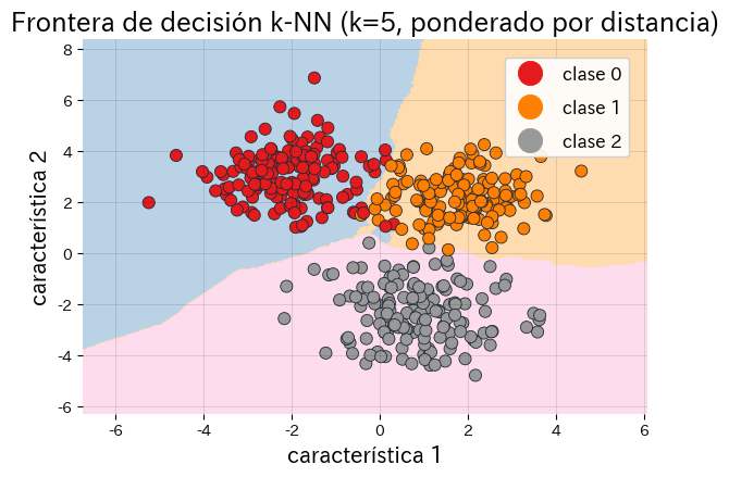
Representa de forma natural fronteras de decisión no lineales, aunque las distancias pierden contraste en alta dimensión (“la maldición de la dimensionalidad”).
Estandarizar las características o seleccionar las más relevantes estabiliza los cálculos de distancia.

Intuición #

Bajo la idea de que “muestras cercanas comparten etiqueta”, k-NN busca los $k$ ejemplos de entrenamiento más próximos al punto objetivo y decide la clase por mayoría (opcionalmente ponderada por la distancia). Como no entrena un modelo explícito de antemano, se le conoce como aprendizaje perezoso.

Formulación matemática #

Para un punto de prueba $\mathbf{x}$, sea $\mathcal{N}_k(\mathbf{x})$ el conjunto de los $k$ vecinos más cercanos. El voto para la clase $c$ es

$$ v_c = \sum_{i \in \mathcal{N}_k(\mathbf{x})} w_i ,\mathbb{1}(y_i = c), $$

donde los pesos $w_i$ pueden ser uniformes o funciones de la distancia (inversa, gaussiana, etc.). La clase con mayor voto se predice como resultado.

Experimentos con Python #

El siguiente código evalúa distintos valores de $k$ con un conjunto de validación y dibuja las regiones de decisión del mejor modelo.

from __future__ import annotations

import japanize_matplotlib
import matplotlib.pyplot as plt
import numpy as np
from matplotlib.colors import ListedColormap
from sklearn.datasets import make_blobs
from sklearn.neighbors import KNeighborsClassifier
from sklearn.pipeline import make_pipeline
from sklearn.preprocessing import StandardScaler


def run_knn_demo(
    n_samples: int = 600,
    random_state: int = 7,
    weights: str = "distance",
    k_values: tuple[int, ...] = (1, 3, 5, 7, 11),
    validation_ratio: float = 0.3,
    title: str = "Regiones de decisión k-NN",
    xlabel: str = "característica 1",
    ylabel: str = "característica 2",
    class_label_prefix: str = "clase",
) -> dict[str, object]:
    """Evaluate k-NN for several neighbour counts and plot decision regions.

    Args:
        n_samples: Number of synthetic samples to draw.
        random_state: Seed for reproducible sampling.
        weights: Weighting scheme handed to KNeighborsClassifier.
        k_values: Candidate neighbour counts to evaluate.
        validation_ratio: Fraction of the data reserved for validation.
        title: Title for the generated figure.
        xlabel: Label for the x-axis.
        ylabel: Label for the y-axis.
        class_label_prefix: Prefix used when labelling the classes.

    Returns:
        Dictionary with validation scores per k and the best-performing k.
    """
    japanize_matplotlib.japanize()
    X, y = make_blobs(
        n_samples=n_samples,
        centers=3,
        cluster_std=[1.1, 1.0, 1.2],
        random_state=random_state,
    )

    rng = np.random.default_rng(random_state)
    indices = rng.permutation(len(X))
    split = int(len(X) * (1.0 - validation_ratio))
    train_idx, valid_idx = indices[:split], indices[split:]
    X_train, X_valid = X[train_idx], X[valid_idx]
    y_train, y_valid = y[train_idx], y[valid_idx]

    scores: dict[int, float] = {}
    for k in k_values:
        model = make_pipeline(
            StandardScaler(),
            KNeighborsClassifier(n_neighbors=k, weights=weights),
        )
        model.fit(X_train, y_train)
        scores[k] = float(model.score(X_valid, y_valid))

    best_k = max(scores, key=scores.get)
    best_model = make_pipeline(
        StandardScaler(),
        KNeighborsClassifier(n_neighbors=best_k, weights=weights),
    )
    best_model.fit(X, y)

    xx, yy = np.meshgrid(
        np.linspace(X[:, 0].min() - 1.5, X[:, 0].max() + 1.5, 300),
        np.linspace(X[:, 1].min() - 1.5, X[:, 1].max() + 1.5, 300),
    )
    grid = np.column_stack([xx.ravel(), yy.ravel()])
    predictions = best_model.predict(grid).reshape(xx.shape)

    unique_classes = np.unique(y)
    levels = np.arange(unique_classes.min(), unique_classes.max() + 2) - 0.5
    cmap = ListedColormap(["#fee0d2", "#deebf7", "#c7e9c0"])

    fig, ax = plt.subplots(figsize=(7, 5.5))
    contour = ax.contourf(xx, yy, predictions, levels=levels, cmap=cmap, alpha=0.85)
    scatter = ax.scatter(
        X[:, 0],
        X[:, 1],
        c=y,
        cmap="Set1",
        edgecolor="#1f2937",
        linewidth=0.6,
    )
    ax.set_title(f"{title} (k={best_k}, weights={weights})")
    ax.set_xlabel(xlabel)
    ax.set_ylabel(ylabel)
    ax.set_xlim(xx.min(), xx.max())
    ax.set_ylim(yy.min(), yy.max())
    ax.grid(alpha=0.15)

    legend = ax.legend(
        handles=scatter.legend_elements()[0],
        labels=[f"{class_label_prefix} {cls}" for cls in unique_classes],
        loc="upper right",
        frameon=True,
    )
    legend.get_frame().set_alpha(0.9)
    fig.colorbar(contour, ax=ax, label="Clase predicha")
    fig.tight_layout()
    plt.show()

    return {"scores": scores, "best_k": int(best_k), "validation_accuracy": scores[best_k]}


metrics = run_knn_demo(
    title="Regiones de decisión k-NN",
    xlabel="característica 1",
    ylabel="característica 2",
    class_label_prefix="clase",
)
print(f"Mejor k: {metrics['best_k']}")
print(f"Precisión de validación (mejor k): {metrics['validation_accuracy']:.3f}")
for candidate_k, score in metrics["scores"].items():
    print(f"k={candidate_k}: precisión de validación={score:.3f}")

Regiones de decisión k-NN

Referencias #

Cover, T. M., & Hart, P. E. (1967). Nearest Neighbor Pattern Classification. IEEE Transactions on Information Theory, 13(1), 21–27.
Hastie, T., Tibshirani, R., & Friedman, J. (2009). The Elements of Statistical Learning. Springer.