2.4.3
Adaboost (clasificación)
Resumen- AdaBoost en clasificación entrena aprendices débiles de forma secuencial y aumenta el peso de los errores previos.
learning_rate y n_estimators determinan la velocidad de ajuste y el equilibrio sesgo-varianza.- Con árboles poco profundos como base, el ensamble corrige gradualmente regiones de decisión difíciles.
Intuicion
#
La idea clave de AdaBoost es volver sobre los errores. Cada clasificador débil aporta una corrección parcial y la combinación ponderada de esas correcciones construye un clasificador final mucho más robusto.
Explicacion Detallada
#
1
2
3
4
5
6
7
8
9
| import matplotlib.pyplot as plt
import japanize_matplotlib
import numpy as np
from sklearn.datasets import make_classification
from sklearn.model_selection import train_test_split
from sklearn.metrics import roc_auc_score
from sklearn.tree import DecisionTreeClassifier
from sklearn.ensemble import AdaBoostClassifier
|
Crear datos para el experimento
#
 1
 2
 3
 4
 5
 6
 7
 8
 9
10
11
12
| n_features = 20
X, y = make_classification(
n_samples=2500,
n_features=n_features,
n_informative=10,
n_classes=2,
n_redundant=4,
n_clusters_per_class=5,
)
X_train, X_test, y_train, y_test = train_test_split(
X, y, test_size=0.33, random_state=42
)
|
Entrenar Adaboost
#
Aquí usamos un árbol de decisión como un aprendiz débil.
 1
 2
 3
 4
 5
 6
 7
 8
 9
10
11
12
| ab_clf = AdaBoostClassifier(
n_estimators=10,
learning_rate=1.0,
random_state=117117,
base_estimator=DecisionTreeClassifier(max_depth=2),
)
ab_clf.fit(X_train, y_train)
y_pred = ab_clf.predict(X_test)
ab_clf_score = roc_auc_score(y_test, y_pred)
ab_clf_score
|
0.7546477034876885
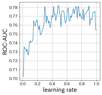
Influencia de la tasa de aprendizaje
#
Cuanto menor sea la tasa de aprendizaje, menor será el rango de las actualizaciones de pesos. Por el contrario, si es demasiado grande, es posible que no ocurra la convergencia.
 1
 2
 3
 4
 5
 6
 7
 8
 9
10
11
12
13
| scores = []
learning_rate_list = np.linspace(0.01, 1, 100)
for lr in learning_rate_list:
ab_clf_i = AdaBoostClassifier(
n_estimators=10,
learning_rate=lr,
random_state=117117,
base_estimator=DecisionTreeClassifier(max_depth=2),
)
ab_clf_i.fit(X_train, y_train)
y_pred = ab_clf_i.predict(X_test)
scores.append(roc_auc_score(y_test, y_pred))
|
1
2
3
4
5
6
| plt.figure(figsize=(5, 5))
plt.plot(learning_rate_list, scores)
plt.xlabel("learning rate")
plt.ylabel("ROC-AUC")
plt.grid()
plt.show()
|
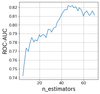
Influencia de n_estimators
#
N_estimators especifica el número de aprendices débiles.
Normalmente, no es necesario hacer este parámetro más grande o más pequeño.
Fija n_estimators en un número grande y luego ajusta los demás parámetros.
 1
 2
 3
 4
 5
 6
 7
 8
 9
10
11
12
13
| scores = []
n_estimators_list = [int(ne) for ne in np.linspace(5, 70, 40)]
for n_estimators in n_estimators_list:
ab_clf_i = AdaBoostClassifier(
n_estimators=int(n_estimators),
learning_rate=0.6,
random_state=117117,
base_estimator=DecisionTreeClassifier(max_depth=2),
)
ab_clf_i.fit(X_train, y_train)
y_pred = ab_clf_i.predict(X_test)
scores.append(roc_auc_score(y_test, y_pred))
|
1
2
3
4
5
6
| plt.figure(figsize=(5, 5))
plt.plot(n_estimators_list, scores)
plt.xlabel("n_estimators")
plt.ylabel("ROC-AUC")
plt.grid()
plt.show()
|
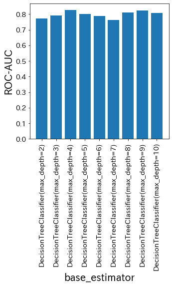
Influencia del base-estimator
#
base_estimator especifica qué usar como aprendiz débil. En otras palabras, es uno de los parámetros más importantes en Adaboost.
 1
 2
 3
 4
 5
 6
 7
 8
 9
10
11
12
13
14
15
| scores = []
base_estimator_list = [
DecisionTreeClassifier(max_depth=md) for md in [2, 3, 4, 5, 6, 7, 8, 9, 10]
]
for base_estimator in base_estimator_list:
ab_clf_i = AdaBoostClassifier(
n_estimators=10,
learning_rate=0.5,
random_state=117117,
base_estimator=base_estimator,
)
ab_clf_i.fit(X_train, y_train)
y_pred = ab_clf_i.predict(X_test)
scores.append(roc_auc_score(y_test, y_pred))
|
1
2
3
4
5
6
7
| plt.figure(figsize=(5, 5))
plt_index = [i for i in range(len(base_estimator_list))]
plt.bar(plt_index, scores)
plt.xticks(plt_index, [str(bm) for bm in base_estimator_list], rotation=90)
plt.xlabel("base_estimator")
plt.ylabel("ROC-AUC")
plt.show()
|
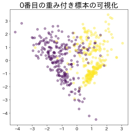
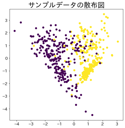
Visualización de los pesos de los datos en Adaboost
#
Visualiza la asignación de pesos a los datos que son difíciles de clasificar.
 1
 2
 3
 4
 5
 6
 7
 8
 9
10
11
12
13
14
15
16
17
18
19
20
21
22
23
24
25
26
27
28
29
30
31
32
33
34
35
36
37
38
39
40
41
42
43
44
| # NOTA: Modelo creado para verificar el sample_weight pasado al modelo
# Este DummyClassifier no cambia los parámetros del Adaboost
class DummyClassifier:
def __init__(self):
self.model = DecisionTreeClassifier(max_depth=3)
self.n_classes_ = 2
self.classes_ = ["A", "B"]
self.sample_weight = None ## sample_weight
def fit(self, X, y, sample_weight=None):
self.sample_weight = sample_weight
self.model.fit(X, y, sample_weight=sample_weight)
return self.model
def predict(self, X, check_input=True):
proba = self.model.predict(X)
return proba
def get_params(self, deep=False):
return {}
def set_params(self, deep=False):
return {}
n_samples = 500
X_2, y_2 = make_classification(
n_samples=n_samples,
n_features=2,
n_informative=2,
n_redundant=0,
n_repeated=0,
random_state=117,
n_clusters_per_class=2,
)
plt.figure(
figsize=(
7,
7,
)
)
plt.title(f"Scatter plots of sample data")
plt.scatter(X_2[:, 0], X_2[:, 1], c=y_2)
plt.show()
|
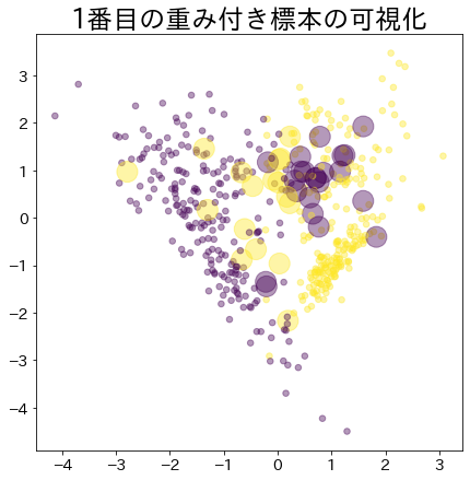
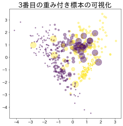
Peso después de que el proceso de arranque ha avanzado
#
Los datos con mayor peso se representan con un círculo más grande.
 1
 2
 3
 4
 5
 6
 7
 8
 9
10
11
12
13
14
15
16
17
18
19
20
21
22
| clf = AdaBoostClassifier(
n_estimators=4, random_state=0, algorithm="SAMME", base_estimator=DummyClassifier()
)
clf.fit(X_2, y_2)
for i, estimators_i in enumerate(clf.estimators_):
plt.figure(
figsize=(
7,
7,
)
)
plt.title(f"Visualization of the {i}-th weighted sample")
plt.scatter(
X_2[:, 0],
X_2[:, 1],
marker="o",
c=y_2,
alpha=0.4,
s=estimators_i.sample_weight * n_samples ** 1.65,
)
plt.show()
|