Regresión Partial Least Squares (PLS)

Actualizado 2020-05-20 Lectura 4 min

Resumen

PLS extrae factores latentes que maximizan la covarianza entre predictores y objetivo antes de realizar la regresión.
A diferencia de PCA, los ejes aprendidos incorporan información de la variable objetivo, manteniendo el desempeño predictivo mientras se reduce la dimensionalidad.
Ajustar el número de factores latentes estabiliza el modelo cuando existe fuerte multicolinealidad.
Analizar los loadings permite identificar qué combinaciones de características se relacionan más con la variable objetivo.

Intuicion #

Este metodo se entiende mejor al conectar sus supuestos con la estructura de los datos y su efecto en la generalizacion.

Explicacion Detallada #

Formulación matemática #

Dado un matriz de predictores $\mathbf{X}$ y un vector objetivo $\mathbf{y}$, PLS alterna las actualizaciones de las puntuaciones latentes $\mathbf{t} = \mathbf{X} \mathbf{w}$ y $\mathbf{u} = \mathbf{y} c$ de forma que la covarianza $\mathbf{t}^\top \mathbf{u}$ sea máxima. Repetir el proceso produce un conjunto de factores latentes sobre el que se ajusta un modelo lineal

$$ \hat{y} = \mathbf{t} \boldsymbol{b} + b_0. $$

El número de factores $k$ suele elegirse mediante validación cruzada.

Experimentos con Python #

Comparamos el desempeño de PLS para distintos números de factores latentes con el conjunto de datos de acondicionamiento físico de Linnerud.

 1
 2
 3
 4
 5
 6
 7
 8
 9
10
11
12
13
14
15
16
17
18
19
20
21
22
23
24
25
26
27
28
29
30
31
32
33
34
35
36
37
38
39
40
41
42
43
44
45
46
47
48
49
50
51
52
53
54
55
56
57
58
59
60
61
62
63
64
65
66
67
68
69
70
71
72
73
74
75
76
77
78
79
80
81
82
83
84
85
86
87
88
89
90
91
92
93
94
95
from __future__ import annotations

import japanize_matplotlib
import matplotlib.pyplot as plt
import numpy as np
from sklearn.cross_decomposition import PLSRegression
from sklearn.datasets import load_linnerud
from sklearn.model_selection import KFold, cross_val_score
from sklearn.pipeline import Pipeline
from sklearn.preprocessing import StandardScaler

def evaluate_pls_latent_factors(
    cv_splits: int = 5,
    xlabel: str = "Number of latent factors",
    ylabel: str = "CV MSE (lower is better)",
    label_best: str = "best={k}",
    title: str | None = None,
) -> dict[str, object]:
    """Cross-validate PLS regression for different latent factor counts.

    Args:
        cv_splits: Number of folds for cross-validation.
        xlabel: Label for the number-of-factors axis.
        ylabel: Label for the cross-validation error axis.
        label_best: Format string for the best-factor annotation.
        title: Optional plot title.

    Returns:
        Dictionary with the selected factor count, CV score, and loadings.
    """
    japanize_matplotlib.japanize()
    data = load_linnerud()
    X = data["data"]
    y = data["target"][:, 0]

    max_components = min(X.shape[1], 6)
    components = np.arange(1, max_components + 1)
    cv = KFold(n_splits=cv_splits, shuffle=True, random_state=0)

    scores = []
    pipelines = []
    for k in components:
        model = Pipeline([
            ("scale", StandardScaler()),
            ("pls", PLSRegression(n_components=int(k))),
        ])
        cv_score = cross_val_score(
            model,
            X,
            y,
            cv=cv,
            scoring="neg_mean_squared_error",
        ).mean()
        scores.append(cv_score)
        pipelines.append(model)

    scores_arr = np.array(scores)
    best_idx = int(np.argmax(scores_arr))
    best_k = int(components[best_idx])
    best_mse = float(-scores_arr[best_idx])

    best_model = pipelines[best_idx].fit(X, y)
    x_loadings = best_model["pls"].x_loadings_
    y_loadings = best_model["pls"].y_loadings_

    fig, ax = plt.subplots(figsize=(8, 4))
    ax.plot(components, -scores_arr, marker="o")
    ax.axvline(best_k, color="red", linestyle="--", label=label_best.format(k=best_k))
    ax.set_xlabel(xlabel)
    ax.set_ylabel(ylabel)
    if title:
        ax.set_title(title)
    ax.legend()
    fig.tight_layout()
    plt.show()

    return {
        "best_k": best_k,
        "best_mse": best_mse,
        "x_loadings": x_loadings,
        "y_loadings": y_loadings,
    }

metrics = evaluate_pls_latent_factors(
    xlabel="Número de factores latentes",
    ylabel="MSE de CV (más bajo es mejor)",
    label_best="mejor k={k}",
    title="Selección de factores en PLS",
)
print(f"Mejor número de factores: {metrics['best_k']}")
print(f"Mejor MSE de CV: {metrics['best_mse']:.3f}")
print("Cargas de X:
", metrics['x_loadings'])
print("Cargas de Y:
", metrics['y_loadings'])

Comparamos el desempeño de PLS para distintos números de fac… (figura)

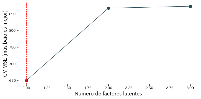
Interpretación de los resultados #

El MSE de validación cruzada desciende al añadir factores, alcanza un mínimo y luego empeora si seguimos agregando más.
Inspeccionar x_loadings_ y y_loadings_ muestra qué características contribuyen más a cada factor latente.
Estandarizar las entradas garantiza que características con diferentes escalas aporten de manera equilibrada.

Referencias #

Wold, H. (1975). Soft Modelling by Latent Variables: The Non-Linear Iterative Partial Least Squares (NIPALS) Approach. En Perspectives in Probability and Statistics. Academic Press.
Geladi, P., & Kowalski, B. R. (1986). Partial Least-Squares Regression: A Tutorial. Analytica Chimica Acta, 185, 1–17.