Regresión polinómica

まとめ

La regresión polinómica amplía las características con potencias para que un modelo lineal pueda ajustar relaciones no lineales.
El modelo sigue siendo una combinación lineal de coeficientes, por lo que mantiene soluciones cerradas e interpretabilidad.
A mayor grado mayor expresividad, pero también riesgo de sobreajuste; por ello la regularización y la validación cruzada son esenciales.
Estandarizar las características y ajustar el grado junto con la penalización produce predicciones estables.

Intuición #

Una recta no puede describir curvas suaves o patrones en forma de colina. Al expandir la entrada con términos polinómicos—$x, x^2, x^3, \dots$ en el caso univariado o potencias e interacciones en el multivariado—expresamos comportamientos no lineales sin abandonar el marco lineal.

Formulación matemática #

Para $\mathbf{x} = (x_1, \dots, x_m)$ generamos un vector de características polinómicas $\phi(\mathbf{x})$ hasta el grado $d$. Por ejemplo, si $m = 2$ y $d = 2$,

$$ \phi(\mathbf{x}) = (1, x_1, x_2, x_1^2, x_1 x_2, x_2^2), $$

y el modelo queda

$$ y = \mathbf{w}^\top \phi(\mathbf{x}). $$

Como el número de términos crece rápidamente con el grado, en la práctica se comienza con grados bajos (2 o 3) y se combina con regularización (p. ej., Ridge) cuando hace falta.

Experimentos con Python #

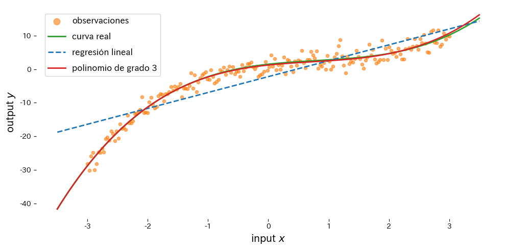
Añadimos características de grado tres y ajustamos una curva a datos generados a partir de una función cúbica con ruido.

from __future__ import annotations

import japanize_matplotlib
import matplotlib.pyplot as plt
import numpy as np
from sklearn.linear_model import LinearRegression
from sklearn.metrics import mean_squared_error
from sklearn.pipeline import make_pipeline
from sklearn.preprocessing import PolynomialFeatures


def compare_polynomial_regression(
    n_samples: int = 200,
    degree: int = 3,
    noise_scale: float = 2.0,
    label_observations: str = "observations",
    label_true_curve: str = "true curve",
    label_linear: str = "linear regression",
    label_poly_template: str = "degree-{degree} polynomial",
) -> tuple[float, float]:
    """Fit linear vs. polynomial regression to a cubic trend and plot the results.

    Args:
        n_samples: Number of synthetic samples generated along the curve.
        degree: Polynomial degree used in the feature expansion.
        noise_scale: Standard deviation of the Gaussian noise added to targets.
        label_observations: Legend label for scatter observations.
        label_true_curve: Legend label for the underlying true curve.
        label_linear: Legend label for the linear regression fit.
        label_poly_template: Format string for the polynomial label.

    Returns:
        A tuple containing the mean-squared errors of (linear, polynomial) models.
    """
    japanize_matplotlib.japanize()
    rng = np.random.default_rng(seed=42)

    x: np.ndarray = np.linspace(-3.0, 3.0, n_samples, dtype=float)
    y_true: np.ndarray = 0.5 * x**3 - 1.2 * x**2 + 2.0 * x + 1.5
    y_noisy: np.ndarray = y_true + rng.normal(scale=noise_scale, size=x.shape)

    X: np.ndarray = x[:, np.newaxis]

    linear_model = LinearRegression()
    linear_model.fit(X, y_noisy)
    poly_model = make_pipeline(
        PolynomialFeatures(degree=degree, include_bias=False),
        LinearRegression(),
    )
    poly_model.fit(X, y_noisy)

    grid: np.ndarray = np.linspace(-3.5, 3.5, 300, dtype=float)[:, np.newaxis]
    linear_pred: np.ndarray = linear_model.predict(grid)
    poly_pred: np.ndarray = poly_model.predict(grid)
    true_curve: np.ndarray = (
        0.5 * grid.ravel()**3 - 1.2 * grid.ravel()**2 + 2.0 * grid.ravel() + 1.5
    )

    linear_mse: float = float(mean_squared_error(y_noisy, linear_model.predict(X)))
    poly_mse: float = float(mean_squared_error(y_noisy, poly_model.predict(X)))

    fig, ax = plt.subplots(figsize=(10, 5))
    ax.scatter(
        X,
        y_noisy,
        s=20,
        color="#ff7f0e",
        alpha=0.6,
        label=label_observations,
    )
    ax.plot(
        grid,
        true_curve,
        color="#2ca02c",
        linewidth=2,
        label=label_true_curve,
    )
    ax.plot(
        grid,
        linear_pred,
        color="#1f77b4",
        linestyle="--",
        linewidth=2,
        label=label_linear,
    )
    ax.plot(
        grid,
        poly_pred,
        color="#d62728",
        linewidth=2,
        label=label_poly_template.format(degree=degree),
    )
    ax.set_xlabel("input $x$")
    ax.set_ylabel("output $y$")
    ax.legend()
    fig.tight_layout()
    plt.show()

    return linear_mse, poly_mse



degree = 3
linear_mse, poly_mse = compare_polynomial_regression(
    degree=degree,
    label_observations="observaciones",
    label_true_curve="curva real",
    label_linear="regresión lineal",
    label_poly_template="polinomio de grado {degree}",
)
print(f"MSE de la regresión lineal: {linear_mse:.3f}")
print(f"MSE del polinomio de grado {degree}: {poly_mse:.3f}")

polynomial-regression block 1

Interpretación de los resultados #

La regresión lineal simple falla en reproducir la curvatura, especialmente cerca del centro, mientras que el modelo cúbico sigue la curva verdadera.
Subir el grado mejora el ajuste en entrenamiento pero puede volver inestables las extrapolaciones.
Combinar características polinómicas con una regresión regularizada (p. ej., Ridge) en una tubería ayuda a controlar el sobreajuste.

Referencias #

Bishop, C. M. (2006). Pattern Recognition and Machine Learning. Springer.
Hastie, T., Tibshirani, R., & Friedman, J. (2009). The Elements of Statistical Learning. Springer.