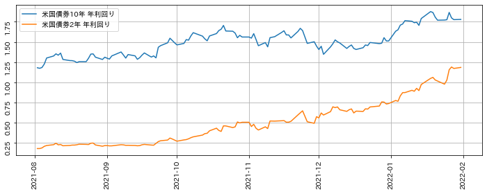
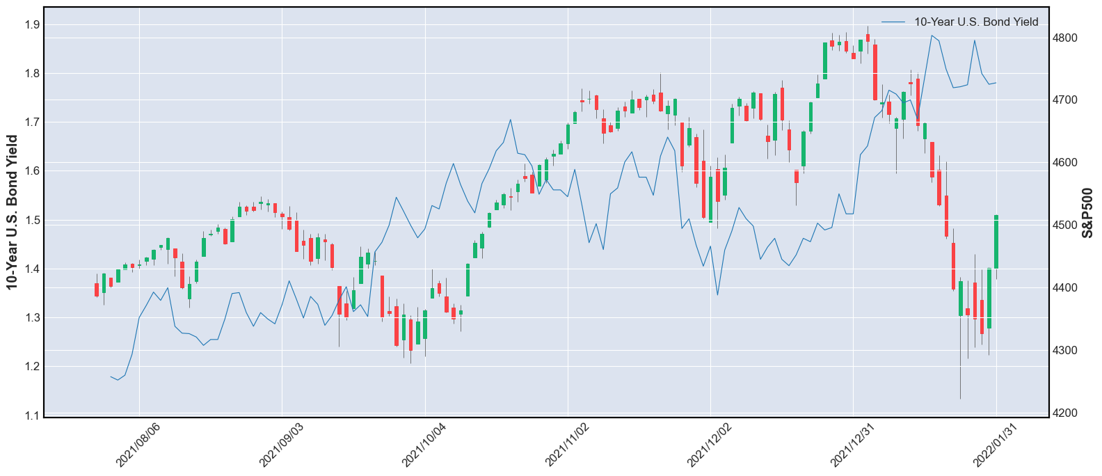
まとめ VOO・VTIなどの代表的なETFの価格推移を取得し、チャートで比較する。 米国債(10年・2年)の利回りデータを取得し、株式市場との関連を分析する。 ローソク足チャートと利回りカーブを重ねて、マクロ環境と株価の連動を確認する。 代表的なETFと債券利回りの推移を比較します。データはstooq から取得しています。
メディアプログラミング入門 WebスクレイピングとWebAPI の講義資料45pで紹介されていたPandas Datareaderを使用しています。
1
2
3
4
5
6
import numpy as np
import pandas as pd
import pandas_datareader.data as web
import matplotlib.pyplot as plt
from IPython.display import display , HTML
from utils import get_finance_data , get_rsi
ETF
# 1
2
3
4
5
6
7
8
9
10
11
12
13
14
15
16
17
18
19
20
# 銘柄名、期間、保存先ファイル
start = "2021-08-01"
end = "2022-01-31"
# データを取得する
voo = get_finance_data ( "VOO" , source = "stooq" , start = start , end = end )
display ( HTML ( f "<h3>VOO</h3>" ))
display ( voo . head ())
vti = get_finance_data ( "VTI" , source = "stooq" , start = start , end = end )
display ( HTML ( f "<h3>VTI</h3>" ))
display ( vti . head ())
spx = get_finance_data ( "^SPX" , source = "stooq" , start = start , end = end )
display ( HTML ( f "<h3>S&P500</h3>" ))
display ( spx . head ())
ndq = get_finance_data ( "^NDQ" , source = "stooq" , start = start , end = end )
display ( HTML ( f "<h3>Nasdaq</h3>" ))
display ( ndq . head ())
VOO Open High Low Close Volume Date 2022-01-31 405.67 413.9700 404.3500 413.69 9200435 2022-01-28 397.82 406.3300 393.3000 406.26 12096807 2022-01-27 402.93 405.9700 394.8200 396.54 12455226 2022-01-26 405.66 408.1954 394.3400 398.56 14377346 2022-01-25 398.17 404.2600 392.7325 399.46 16836326
VTI Open High Low Close Volume Date 2022-01-31 222.09 226.950 221.22 226.81 5306436 2022-01-28 217.50 222.170 214.93 222.09 4961209 2022-01-27 220.81 222.400 215.90 216.75 5791524 2022-01-26 222.72 224.160 216.05 218.37 7096416 2022-01-25 219.10 222.015 215.64 219.22 6600378
S&P500 Open High Low Close Volume Date 2022-01-31 4431.79 4516.89 4414.02 4515.55 2960132803 2022-01-28 4336.19 4432.72 4292.46 4431.85 2926083817 2022-01-27 4380.58 4428.74 4309.50 4326.51 3070684348 2022-01-26 4408.43 4453.23 4304.80 4349.93 3239353450 2022-01-25 4366.64 4411.01 4287.11 4356.45 3069079477
Nasdaq Open High Low Close Volume Date 2022-01-31 13812.20 14242.90 13767.71 14239.88 3268652504 2022-01-28 13436.71 13771.91 13236.55 13770.57 3092819850 2022-01-27 13710.99 13765.91 13322.66 13352.78 3373437394 2022-01-26 13871.77 14002.65 13392.19 13542.12 3664304374 2022-01-25 13610.87 13781.63 13414.14 13539.29 3265336637
債権利回り
# 1
2
3
4
5
6
7
usy10 = get_finance_data ( "10USY.B" , source = "stooq" , start = start , end = end )
display ( HTML ( f "<h3>10-Year U.S. Bond Yield</h3>" ))
display ( usy10 . head ())
usy2 = get_finance_data ( "2USY.B" , source = "stooq" , start = start , end = end )
display ( HTML ( f "<h3>2-Year U.S. Bond Yield</h3>" ))
display ( usy2 . head ())
10-Year U.S. Bond Yield Open High Low Close Date 2022-01-31 1.789 1.816 1.771 1.780 2022-01-28 1.830 1.848 1.773 1.777 2022-01-27 1.840 1.851 1.783 1.799 2022-01-26 1.769 1.876 1.769 1.867 2022-01-25 1.753 1.792 1.735 1.776
2-Year U.S. Bond Yield Open High Low Close Date 2022-01-31 1.1986 1.2145 1.1587 1.1827 2022-01-28 1.2141 1.2260 1.1603 1.1703 2022-01-27 1.1822 1.2061 1.1603 1.1882 2022-01-26 1.0313 1.1603 1.0154 1.1544 2022-01-25 1.0055 1.0353 0.9897 1.0254
1
2
3
4
5
6
7
plt . figure ( figsize = ( 12 , 4 ))
plt . plot ( usy10 . Close , label = "米国債券10年 年利回り" )
plt . plot ( usy2 . Close , label = "米国債券2年 年利回り" )
plt . legend ()
plt . tick_params ( rotation = 90 )
plt . grid ()
plt . show ()
S&P500と10年債利回りの比較
# 1
2
3
4
5
6
7
8
9
10
11
12
13
14
15
16
17
18
19
20
21
22
23
import mplfinance as mpf
fig = mpf . figure ( figsize = ( 16 , 7 ), tight_layout = True , style = "default" )
ax1 = fig . add_subplot ( 111 )
ax2 = ax1 . twinx ()
mpf . plot ( spx , type = "candle" , style = "yahoo" , datetime_format = "%Y/%m/ %d " , ax = ax1 )
ax1 . set_ylabel ( "S&P500" )
ax1 . invert_xaxis ()
mpf . plot (
usy10 ,
type = "line" ,
style = "starsandstripes" ,
datetime_format = "%Y/%m/ %d " ,
ax = ax2 ,
)
# 左側にラベルを表示する
ax2 . tick_params ( labelleft = True , labelright = False )
ax2 . set_ylabel ( "10-Year U.S. Bond Yield" )
ax2 . yaxis . set_label_position ( "left" )
ax2 . legend ([ "10-Year U.S. Bond Yield" ])
<matplotlib.legend.Legend at 0x7fcc4de60970>