Linear Discriminant Analysis (LDA)

Diperbarui 2020-03-11 Baca 3 menit

Ringkasan

LDA mencari arah yang memaksimalkan rasio antara variansi antar kelas dan variansi intra kelas, sehingga berguna untuk klasifikasi sekaligus reduksi dimensi.
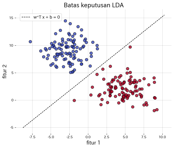
Batas keputusan berbentuk $\mathbf{w}^\top \mathbf{x} + b = 0$; di 2D berupa garis dan di 3D berupa bidang, mudah ditafsirkan secara geometris.
Dengan asumsi tiap kelas berdistribusi Gaussian dan berbagi kovarians yang sama, LDA mendekati klasifikator Bayes optimal.
LinearDiscriminantAnalysis di scikit-learn memudahkan visualisasi batas keputusan dan inspeksi fitur hasil proyeksi.

Intuisi #

Metode ini dipahami lewat asumsi dasarnya, karakteristik data, dan dampak pengaturan parameter terhadap generalisasi.

Penjelasan Rinci #

Formulasi matematis #

Untuk dua kelas, arah proyeksi $\mathbf{w}$ memaksimalkan

$$ J(\mathbf{w}) = \frac{\mathbf{w}^\top \mathbf{S}_B \mathbf{w}}{\mathbf{w}^\top \mathbf{S}_W \mathbf{w}}, $$

di mana $\mathbf{S}_B$ adalah matriks sebar antar kelas dan $\mathbf{S}_W$ adalah matriks sebar intra kelas. Pada kasus multikelas diperoleh hingga $K-1$ arah proyeksi yang berguna untuk reduksi dimensi.

Eksperimen dengan Python #

Contoh berikut menerapkan LDA pada data sintetis dua kelas, menggambar batas keputusan, dan menampilkan fitur hasil proyeksi 1D. Dengan transform, data hasil proyeksi dapat langsung diperoleh.

from __future__ import annotations

import japanize_matplotlib
import matplotlib.pyplot as plt
import numpy as np
from sklearn.datasets import make_blobs
from sklearn.discriminant_analysis import LinearDiscriminantAnalysis
from sklearn.metrics import accuracy_score

def run_lda_demo(
    n_samples: int = 200,
    random_state: int = 42,
    title_boundary: str = "Batas keputusan LDA",
    title_projection: str = "Proyeksi satu dimensi oleh LDA",
    xlabel: str = "fitur 1",
    ylabel: str = "fitur 2",
    hist_xlabel: str = "fitur terproyeksi",
    class0_label: str = "kelas 0",
    class1_label: str = "kelas 1",
) -> dict[str, float]:
    """Train LDA on synthetic blobs and plot boundary plus projection."""
    japanize_matplotlib.japanize()
    X, y = make_blobs(
        n_samples=n_samples,
        centers=2,
        n_features=2,
        cluster_std=2.0,
        random_state=random_state,
    )

    clf = LinearDiscriminantAnalysis(store_covariance=True)
    clf.fit(X, y)

    accuracy = float(accuracy_score(y, clf.predict(X)))
    w = clf.coef_[0]
    b = float(clf.intercept_[0])

    xs = np.linspace(X[:, 0].min() - 1, X[:, 0].max() + 1, 300)
    ys_boundary = -(w[0] / w[1]) * xs - b / w[1]

    fig, ax = plt.subplots(figsize=(7, 6))
    ax.set_title(title_boundary)
    ax.scatter(X[:, 0], X[:, 1], c=y, cmap="coolwarm", edgecolor="k", alpha=0.8)
    ax.plot(xs, ys_boundary, "k--", lw=1.2, label="w^T x + b = 0")
    ax.set_xlabel(xlabel)
    ax.set_ylabel(ylabel)
    ax.legend(loc="best")
    ax.grid(alpha=0.25)
    fig.tight_layout()
    plt.show()

    X_proj = clf.transform(X)[:, 0]

    fig, ax = plt.subplots(figsize=(8, 4))
    ax.set_title(title_projection)
    ax.hist(X_proj[y == 0], bins=20, alpha=0.7, label=class0_label)
    ax.hist(X_proj[y == 1], bins=20, alpha=0.7, label=class1_label)
    ax.set_xlabel(hist_xlabel)
    ax.legend(loc="best")
    ax.grid(alpha=0.25)
    fig.tight_layout()
    plt.show()

    return {"accuracy": accuracy}

metrics = run_lda_demo(
    title_boundary="Batas keputusan LDA",
    title_projection="Proyeksi satu dimensi oleh LDA",
    xlabel="fitur 1",
    ylabel="fitur 2",
    hist_xlabel="fitur terproyeksi",
    class0_label="kelas 0",
    class1_label="kelas 1",
)
print(f"Akurasi pelatihan: {metrics['accuracy']:.3f}")

Dengan transform, data hasil proyeksi dapat langsung diperol… (diagram)

Referensi #

Fisher, R. A. (1936). The Use of Multiple Measurements in Taxonomic Problems. Annals of Eugenics, 7(2), 179–188.
Hastie, T., Tibshirani, R., & Friedman, J. (2009). The Elements of Statistical Learning. Springer.