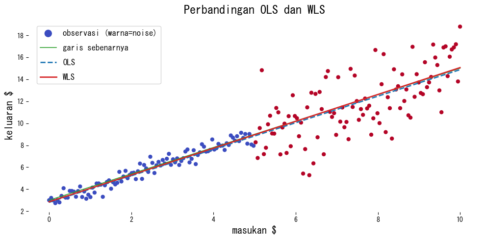
from __future__ import annotations

import japanize_matplotlib
import matplotlib.pyplot as plt
import numpy as np
from sklearn.linear_model import LinearRegression


def run_weighted_vs_ols(
    n_samples: int = 200,
    threshold: float = 5.0,
    low_noise: float = 0.5,
    high_noise: float = 2.5,
    xlabel: str = "input $",
    ylabel: str = "output $",
    label_scatter: str = "observations (color=noise)",
    label_truth: str = "true line",
    label_ols: str = "OLS",
    label_wls: str = "WLS",
    title: str | None = None,
) -> dict[str, float]:
    """Compare OLS and weighted least squares on heteroscedastic data.

    Args:
        n_samples: Number of evenly spaced samples to generate.
        threshold: Breakpoint separating low- and high-noise regions.
        low_noise: Noise scale for the lower region.
        high_noise: Noise scale for the higher region.
        xlabel: Label for the x-axis.
        ylabel: Label for the y-axis.
        label_scatter: Legend label for the colored scatter plot.
        label_truth: Legend label for the ground-truth line.
        label_ols: Legend label for the OLS fit.
        label_wls: Legend label for the WLS fit.
        title: Optional title for the plot.

    Returns:
        Dictionary with slopes and intercepts of both fits.
    """
    japanize_matplotlib.japanize()
    rng = np.random.default_rng(7)

    X_vals: np.ndarray = np.linspace(0.0, 10.0, n_samples, dtype=float)
    true_y: np.ndarray = 1.2 * X_vals + 3.0

    noise_scale = np.where(X_vals < threshold, low_noise, high_noise)
    y_noisy = true_y + rng.normal(scale=noise_scale)

    weights = 1.0 / (noise_scale**2)
    X = X_vals[:, np.newaxis]

    ols = LinearRegression()
    ols.fit(X, y_noisy)

    wls = LinearRegression()
    wls.fit(X, y_noisy, sample_weight=weights)

    grid = np.linspace(0.0, 10.0, 200, dtype=float)[:, np.newaxis]
    ols_pred = ols.predict(grid)
    wls_pred = wls.predict(grid)

    fig, ax = plt.subplots(figsize=(10, 5))
    scatter = ax.scatter(
        X,
        y_noisy,
        c=noise_scale,
        cmap="coolwarm",
        s=25,
        label=label_scatter,
    )
    ax.plot(grid, 1.2 * grid.ravel() + 3.0, color="#2ca02c", label=label_truth)
    ax.plot(grid, ols_pred, color="#1f77b4", linestyle="--", linewidth=2, label=label_ols)
    ax.plot(grid, wls_pred, color="#d62728", linewidth=2, label=label_wls)
    ax.set_xlabel(xlabel)
    ax.set_ylabel(ylabel)
    if title:
        ax.set_title(title)
    ax.legend()
    fig.tight_layout()
    plt.show()

    return {
        "ols_slope": float(ols.coef_[0]),
        "ols_intercept": float(ols.intercept_),
        "wls_slope": float(wls.coef_[0]),
        "wls_intercept": float(wls.intercept_),
    }



metrics = run_weighted_vs_ols(
    xlabel="masukan $",
    ylabel="keluaran $",
    label_scatter="observasi (warna=noise)",
    label_truth="garis sebenarnya",
    label_ols="OLS",
    label_wls="WLS",
    title="Perbandingan OLS dan WLS",
)
print(f"Kemiringan OLS: {metrics['ols_slope']:.3f}, intercept: {metrics['ols_intercept']:.3f}")
print(f"Kemiringan WLS: {metrics['wls_slope']:.3f}, intercept: {metrics['wls_intercept']:.3f}")