Ringkasan- Koefisien korelasiの概要を押さえ、評価対象と読み取り方を整理します。
- Python 3.13 のコード例で算出・可視化し、手順と実務での確認ポイントを確認します。
- 図表や補助指標を組み合わせ、モデル比較や閾値調整に活かすヒントをまとめます。
Koefisien korelasi mengukur kekuatan hubungan linier antara dua data atau variabel acak.
Ini adalah indikator yang memungkinkan kita untuk memeriksa apakah ada perubahan tren bentuk linier antara dua variabel, yang dapat dinyatakan dalam persamaan berikut.
$
\frac{\Sigma_{i=1}^N (x_i - \bar{x})(y_i - \bar{y})}{\sqrt{\Sigma_{i=1}^N(x_i - \bar{x})^2 \Sigma_{i=1}^N(y_i - \bar{y})^2 }}
$
Ini memiliki sifat-sifat berikut
-1 sampai kurang dari 1
Jika koefisien korelasi mendekati 1, \(x\) meningkat → \(y\) juga meningkat
Nilai koefisien korelasi tidak berubah ketika \(x, y\) dikalikan dengan angka yang rendah
Hitung koefisien korelasi antara dua kolom numerik
#
1
2
3
| import numpy as np
np.random.seed(777) # untuk memperbaiki angka acak
|
 1
 2
 3
 4
 5
 6
 7
 8
 9
10
11
12
13
14
15
16
17
| import matplotlib.pyplot as plt
import numpy as np
x = [xi + np.random.rand() for xi in np.linspace(0, 100, 40)]
y = [yi + np.random.rand() for yi in np.linspace(1, 50, 40)]
plt.figure(figsize=(5, 5))
plt.scatter(x, y)
plt.show()
coef = np.corrcoef(x, y)
print(coef)
|
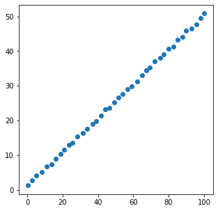
[[1.         0.99979848]

 [0.99979848 1.        ]]
Secara kolektif menghitung koefisien korelasi antara beberapa variabel
#
1
2
3
4
5
| import seaborn as sns
df = sns.load_dataset("iris")
df.head()
|
<tr style="text-align: right;">

  <th></th>

  <th>sepal_length</th>

  <th>sepal_width</th>

  <th>petal_length</th>

  <th>petal_width</th>

  <th>species</th>

</tr>
<tr>

  <th>0</th>

  <td>5.1</td>

  <td>3.5</td>

  <td>1.4</td>

  <td>0.2</td>

  <td>setosa</td>

</tr>

<tr>

  <th>1</th>

  <td>4.9</td>

  <td>3.0</td>

  <td>1.4</td>

  <td>0.2</td>

  <td>setosa</td>

</tr>

<tr>

  <th>2</th>

  <td>4.7</td>

  <td>3.2</td>

  <td>1.3</td>

  <td>0.2</td>

  <td>setosa</td>

</tr>

<tr>

  <th>3</th>

  <td>4.6</td>

  <td>3.1</td>

  <td>1.5</td>

  <td>0.2</td>

  <td>setosa</td>

</tr>

<tr>

  <th>4</th>

  <td>5.0</td>

  <td>3.6</td>

  <td>1.4</td>

  <td>0.2</td>

  <td>setosa</td>

</tr>
Periksa KORELASI KORELASI antara semua variabel
#
Dengan menggunakan dataset iris mata, mari kita lihat korelasi antar variabel.
1
| df.corr().style.background_gradient(cmap="YlOrRd")
|
<tr>
<th class="blank level0" > </th>
<th class="col_heading level0 col0" >sepal_length</th>
<th class="col_heading level0 col1" >sepal_width</th>
<th class="col_heading level0 col2" >petal_length</th>
<th class="col_heading level0 col3" >petal_width</th>
</tr>
<tr>

  <th id="T_dbd76_level0_row0" class="row_heading level0 row0" >sepal_length</th>

  <td id="T_dbd76_row0_col0" class="data row0 col0" >1.000000</td>

  <td id="T_dbd76_row0_col1" class="data row0 col1" >-0.117570</td>

  <td id="T_dbd76_row0_col2" class="data row0 col2" >0.871754</td>

  <td id="T_dbd76_row0_col3" class="data row0 col3" >0.817941</td>

</tr>

<tr>

  <th id="T_dbd76_level0_row1" class="row_heading level0 row1" >sepal_width</th>

  <td id="T_dbd76_row1_col0" class="data row1 col0" >-0.117570</td>

  <td id="T_dbd76_row1_col1" class="data row1 col1" >1.000000</td>

  <td id="T_dbd76_row1_col2" class="data row1 col2" >-0.428440</td>

  <td id="T_dbd76_row1_col3" class="data row1 col3" >-0.366126</td>

</tr>

<tr>

  <th id="T_dbd76_level0_row2" class="row_heading level0 row2" >petal_length</th>

  <td id="T_dbd76_row2_col0" class="data row2 col0" >0.871754</td>

  <td id="T_dbd76_row2_col1" class="data row2 col1" >-0.428440</td>

  <td id="T_dbd76_row2_col2" class="data row2 col2" >1.000000</td>

  <td id="T_dbd76_row2_col3" class="data row2 col3" >0.962865</td>

</tr>

<tr>

  <th id="T_dbd76_level0_row3" class="row_heading level0 row3" >petal_width</th>

  <td id="T_dbd76_row3_col0" class="data row3 col0" >0.817941</td>

  <td id="T_dbd76_row3_col1" class="data row3 col1" >-0.366126</td>

  <td id="T_dbd76_row3_col2" class="data row3 col2" >0.962865</td>

  <td id="T_dbd76_row3_col3" class="data row3 col3" >1.000000</td>

</tr>
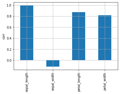
Dalam peta panas, sulit untuk melihat di mana korelasi tertinggi. Periksa diagram batang untuk melihat variabel mana yang memiliki korelasi tertinggi dengan sepal_length.
1
| df.corr()["sepal_length"].plot.bar(grid=True, ylabel="corr")
|
<AxesSubplot:ylabel='corr'>
Ketika koefisien korelasi rendah
#
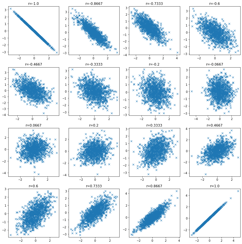
Periksa distribusi data ketika koefisien korelasi rendah dan konfirmasikan bahwa koefisien korelasi mungkin rendah bahkan ketika ada hubungan antar variabel.
 1
 2
 3
 4
 5
 6
 7
 8
 9
10
11
12
13
14
15
16
17
18
19
20
21
22
23
| n_samples = 1000
plt.figure(figsize=(12, 12))
for i, ci in enumerate(np.linspace(-1, 1, 16)):
ci = np.round(ci, 4)
mean = np.array([0, 0])
cov = np.array([[1, ci], [ci, 1]])
v1, v2 = np.random.multivariate_normal(mean, cov, size=n_samples).T
plt.subplot(4, 4, i + 1)
plt.plot(v1, v2, "x")
plt.title(f"r={ci}")
plt.tight_layout()
plt.show()
|
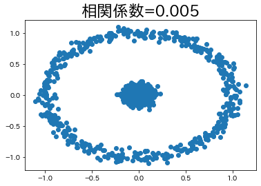
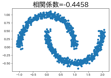
Dalam beberapa kasus, ada hubungan antara variabel bahkan jika koefisien korelasinya rendah.
Kita akan mencoba membuat contoh seperti itu, meskipun sederhana.
 1
 2
 3
 4
 5
 6
 7
 8
 9
10
11
12
13
14
15
16
17
18
19
20
21
22
23
24
25
26
27
| import japanize_matplotlib
from sklearn import datasets
japanize_matplotlib.japanize()
n_samples = 1000
circle, _ = datasets.make_circles(n_samples=n_samples, factor=0.1, noise=0.05)
moon, _ = datasets.make_moons(n_samples=n_samples, noise=0.05)
corr_circle = np.round(np.corrcoef(circle[:, 0], circle[:, 1])[1, 0], 4)
plt.title(f"koefisien korelasi={corr_circle}", fontsize=23)
plt.scatter(circle[:, 0], circle[:, 1])
plt.show()
corr_moon = np.round(np.corrcoef(moon[:, 0], moon[:, 1])[1, 0], 4)
plt.title(f"koefisien korelasi={corr_moon}", fontsize=23)
plt.scatter(moon[:, 0], moon[:, 1])
plt.show()
|