ランダムフォレスト
ランダムフォレストとはアンサンブル学習をするアルゴリズムであり、ランダムに選択した特徴をつかって作成した決定木を組合わせることで汎化能力と予測精度を向上させています。
このページではランダムフォレストを実行した上で、モデルにふくまれる各決定木の性能や中身を確認してみます。
import numpy as np
import matplotlib.pyplot as plt
ランダムフォレストを学習
ROC-AUCについては、ROC-AUCにプロットの仕方について説明を載せています。
from sklearn.datasets import make_classification
from sklearn.ensemble import RandomForestClassifier
from sklearn.model_selection import train_test_split
from sklearn.metrics import roc_auc_score

n_features = 20
X, y = make_classification(
    n_samples=2500,
    n_features=n_features,
    n_informative=10,
    n_classes=2,
    n_redundant=0,
    n_clusters_per_class=4,
    random_state=777,
)
X_train, X_test, y_train, y_test = train_test_split(
    X, y, test_size=0.33, random_state=777
)

model = RandomForestClassifier(
    n_estimators=50, max_depth=3, random_state=777, bootstrap=True, oob_score=True
)
model.fit(X_train, y_train)
y_pred = model.predict(X_test)
rf_score = roc_auc_score(y_test, y_pred)
print(f"テストデータでのROC-AUC = {rf_score}")
テストデータでのROC-AUC = 0.814573097628059
ランダムフォレストに含まれる各木の性能を確認する
import japanize_matplotlib

estimator_scores = []
for i in range(10):
    estimator = model.estimators_[i]
    estimator_pred = estimator.predict(X_test)
    estimator_scores.append(roc_auc_score(y_test, estimator_pred))

plt.figure(figsize=(10, 4))
bar_index = [i for i in range(len(estimator_scores))]
plt.bar(bar_index, estimator_scores)
plt.bar([10], rf_score)
plt.xticks(bar_index + [10], bar_index + ["RF"])
plt.xlabel("木のインデックス")
plt.ylabel("ROC-AUC")
plt.show()
特徴の重要度
不純度(impurity)に基づいた重要度
plt.figure(figsize=(10, 4))
feature_index = [i for i in range(n_features)]
plt.bar(feature_index, model.feature_importances_)
plt.xlabel("特徴のインデックス")
plt.ylabel("特徴の重要度")
plt.show()
permutation importance
from sklearn.inspection import permutation_importance

p_imp = permutation_importance(
    model, X_train, y_train, n_repeats=10, random_state=77
).importances_mean

plt.figure(figsize=(10, 4))
plt.bar(feature_index, p_imp)
plt.xlabel("特徴のインデックス")
plt.ylabel("特徴の重要度")
plt.show()
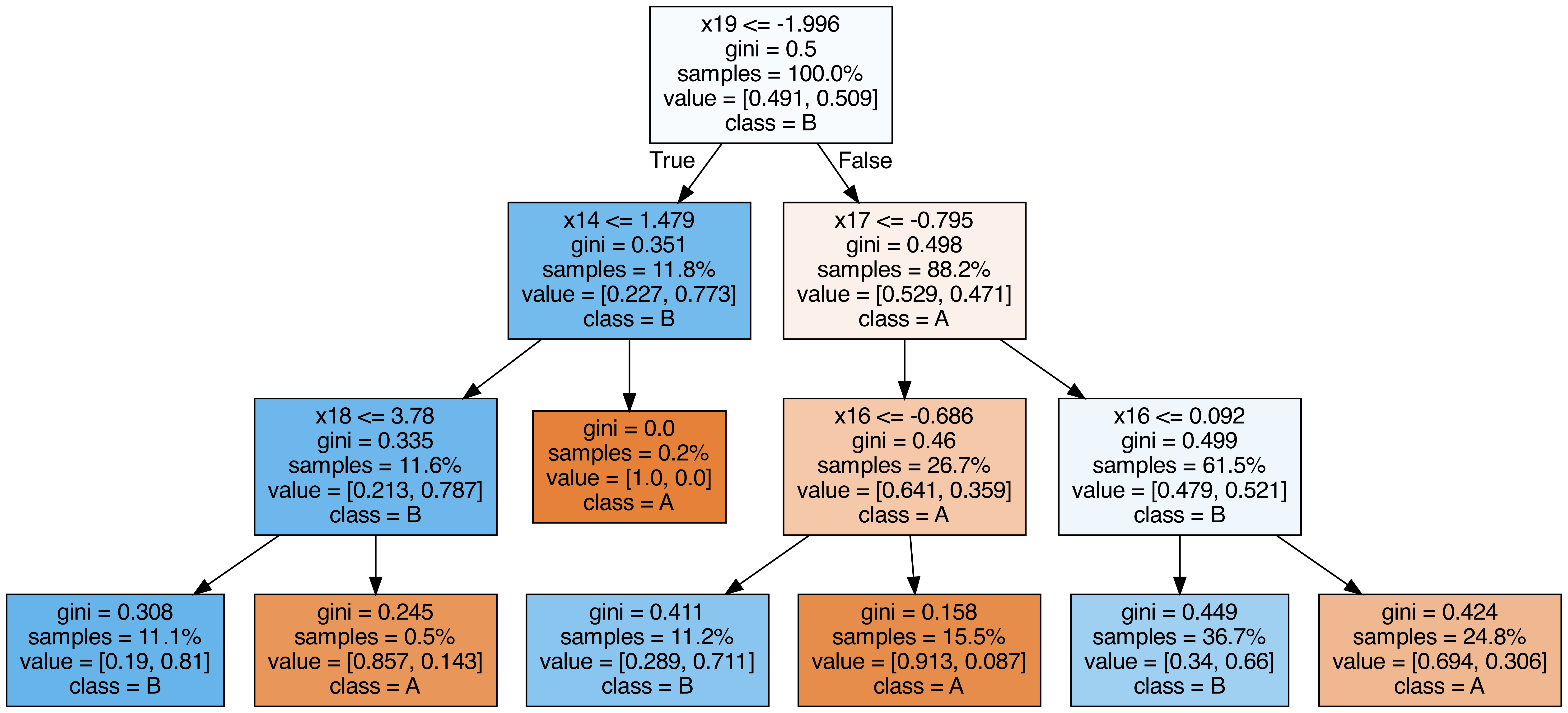
ランダムフォレストに含まれる各木を出力する
from sklearn.tree import export_graphviz
from subprocess import call
from IPython.display import Image
from IPython.display import display

for i in range(10):
    try:
        estimator = model.estimators_[i]
        export_graphviz(
            estimator,
            out_file=f"tree{i}.dot",
            feature_names=[f"x{i}" for i in range(n_features)],
            class_names=["A", "B"],
            proportion=True,
            filled=True,
        )

        call(["dot", "-Tpng", f"tree{i}.dot", "-o", f"tree{i}.png", "-Gdpi=500"])
        display(Image(filename=f"tree{i}.png"))
    except KeyboardInterrupt:
        # TODO: jupyter bookビルド時に出力に失敗するため一時的に例外処理を挟む
        pass
OOB(out-of-bag) Score
OOBによる検証とテストデータでの検証結果が近い値を取ることが確認できます。 乱数と木の深さを変えつつ、OOBでのAccuracyとテストデータでのAccuracyを比較します。
from sklearn.metrics import accuracy_score

for i in range(10):
    model_i = RandomForestClassifier(
        n_estimators=50,
        max_depth=3 + i % 2,
        random_state=i,
        bootstrap=True,
        oob_score=True,
    )
    model_i.fit(X_train, y_train)
    y_pred = model_i.predict(X_test)
    oob_score = model_i.oob_score_
    test_score = accuracy_score(y_test, y_pred)
    print(f"OOBでの検証結果={oob_score} テストデータでの検証結果={test_score}")
OOBでの検証結果=0.786865671641791 テストデータでの検証結果=0.8121212121212121
OOBでの検証結果=0.8101492537313433 テストデータでの検証結果=0.8363636363636363
OOBでの検証結果=0.7886567164179105 テストデータでの検証結果=0.8024242424242424
OOBでの検証結果=0.8161194029850747 テストデータでの検証結果=0.8315151515151515
OOBでの検証結果=0.7910447761194029 テストデータでの検証結果=0.8072727272727273
OOBでの検証結果=0.8101492537313433 テストデータでの検証結果=0.833939393939394
OOBでの検証結果=0.7814925373134328 テストデータでの検証結果=0.8133333333333334
OOBでの検証結果=0.8059701492537313 テストデータでの検証結果=0.833939393939394
OOBでの検証結果=0.7832835820895523 テストデータでの検証結果=0.7951515151515152
OOBでの検証結果=0.8083582089552239 テストデータでの検証結果=0.8387878787878787