決定木のパラメータ

決定木には様々なパラメータが存在し、その指定方法によって結果が変化します。このページでは、それぞれのパラメータがどのような働きをしているか可視化して確認してみようと思います。

max_depthは木の最大深さを指定します
min_samples_splitは分岐を作成するために必要な最低データ数を指定します
min_samples_leafは葉の作成に必要な最低データ数を指定します
max_leaf_nodesは葉の枚数の上限を指定します
ccp_alphaは木の複雑さを考慮した決定木の剪定をするためのパラメタ
class_weightは分類においてクラスの重みづけを指定します

import matplotlib.pyplot as plt
from sklearn.tree import DecisionTreeRegressor
from sklearn.datasets import make_regression
from mpl_toolkits.mplot3d import Axes3D
from dtreeviz.trees import dtreeviz, rtreeviz_bivar_3D

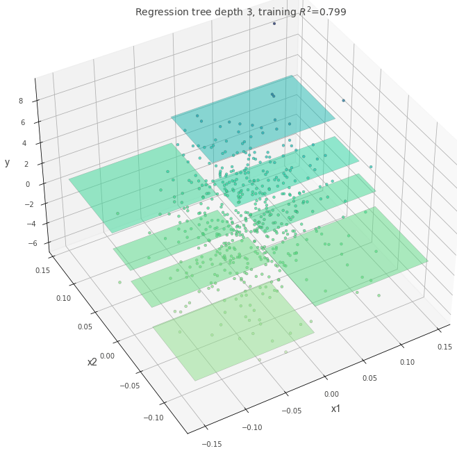
シンプルなデータに決定木を当てはめてみる

# サンプルデータ
X, y = make_regression(n_samples=100, n_features=2, random_state=11)

# 決定木を学習
dt = DecisionTreeRegressor(max_depth=3)
dt.fit(X, y)

# 可視化
fig = plt.figure(figsize=(10, 10))
ax = fig.add_subplot(111, projection="3d")
t = rtreeviz_bivar_3D(
    dt,
    X,
    y,
    feature_names=["x1", "x2"],
    target_name="MPG",
    elev=40,
    azim=120,
    dist=8.0,
    show={"splits", "title"},
    ax=ax,
)
plt.show()

png

いろいろなパラメタの決定木を学習してみる

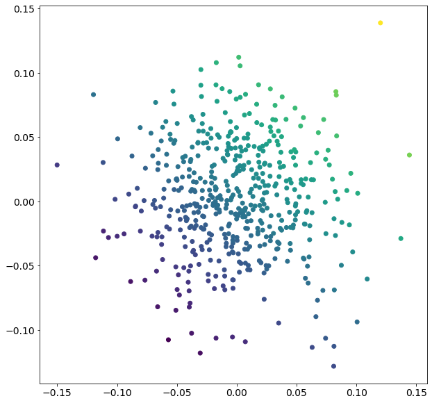
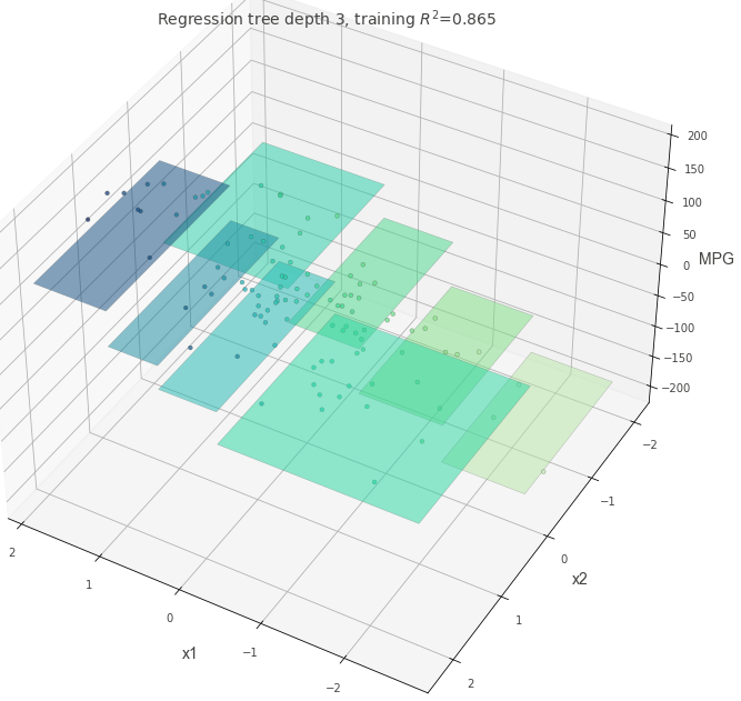
少し複雑な構造を持つデータに対して、決定木のパラメタを変えた時にどのような挙動になるかを確認してみる。はじめに、max_depth=3以外がすべてデフォルト値の決定木を確認する。

# サンプルデータ
X, y = make_regression(
    n_samples=500, n_features=2, effective_rank=4, noise=0.1, random_state=1
)
plt.figure(figsize=(10, 10))
plt.scatter(X[:, 0], X[:, 1], c=y)
plt.show()

# 決定木を学習
dt = DecisionTreeRegressor(max_depth=3, random_state=117117)
dt.fit(X, y)

fig = plt.figure(figsize=(10, 10))
ax = fig.add_subplot(111, projection="3d")
t = rtreeviz_bivar_3D(
    dt,
    X,
    y,
    feature_names=["x1", "x2"],
    target_name="y",
    elev=40,
    azim=240,
    dist=8.0,
    show={"splits", "title"},
    ax=ax,
)
plt.show()

png

max_depth = 10

max_depthの値が大きい時、より深い複雑な木ができます。これは複雑なルールを表現できますが、データ数が少ない場合は過学習している可能性もあります。

dt = DecisionTreeRegressor(max_depth=10, random_state=117117)
dt.fit(X, y)

fig = plt.figure(figsize=(10, 10))
ax = fig.add_subplot(111, projection="3d")
t = rtreeviz_bivar_3D(
    dt,
    X,
    y,
    feature_names=["x1", "x2"],
    target_name="y",
    elev=40,
    azim=240,
    dist=8.0,
    show={"splits", "title"},
    ax=ax,
)
plt.show()

png

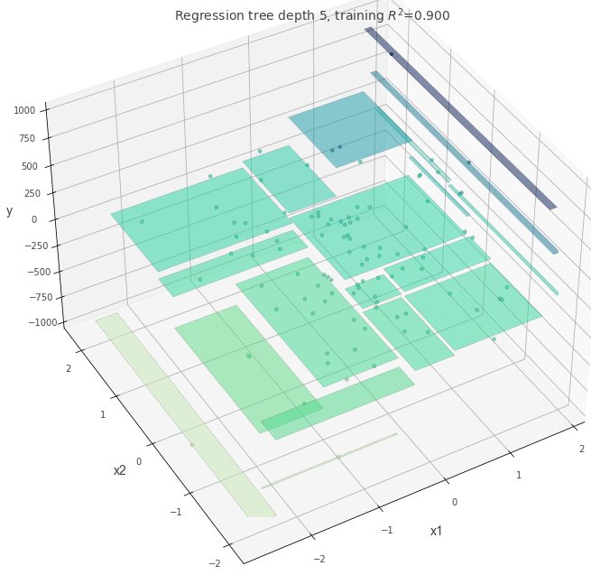
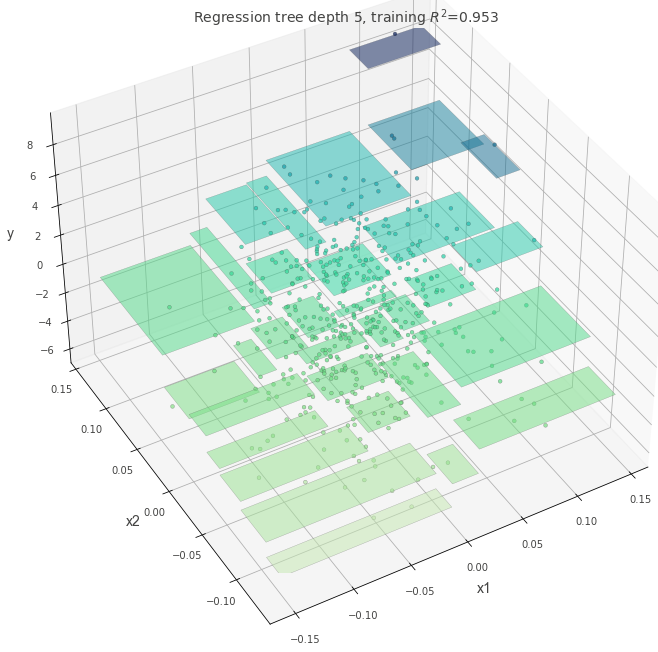
max-depth=5

dt = DecisionTreeRegressor(max_depth=5, random_state=117117)
dt.fit(X, y)

fig = plt.figure(figsize=(10, 10))
ax = fig.add_subplot(111, projection="3d")
t = rtreeviz_bivar_3D(
    dt,
    X,
    y,
    feature_names=["x1", "x2"],
    target_name="y",
    elev=40,
    azim=240,
    dist=8.0,
    show={"splits", "title"},
    ax=ax,
)
plt.show()

png

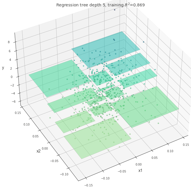
min_samples_split=60

一つの分岐を作るために必要な最低データ数を指定します。 min_samples_split の数を小さくすれば細かいルールを作成できます。大きくすれば過学習は避けられるでしょう。

dt = DecisionTreeRegressor(max_depth=5, min_samples_split=60, random_state=117117)
dt.fit(X, y)

fig = plt.figure(figsize=(10, 10))
ax = fig.add_subplot(111, projection="3d")
t = rtreeviz_bivar_3D(
    dt,
    X,
    y,
    feature_names=["x1", "x2"],
    target_name="y",
    elev=40,
    azim=240,
    dist=8.0,
    show={"splits", "title"},
    ax=ax,
)
plt.show()

png

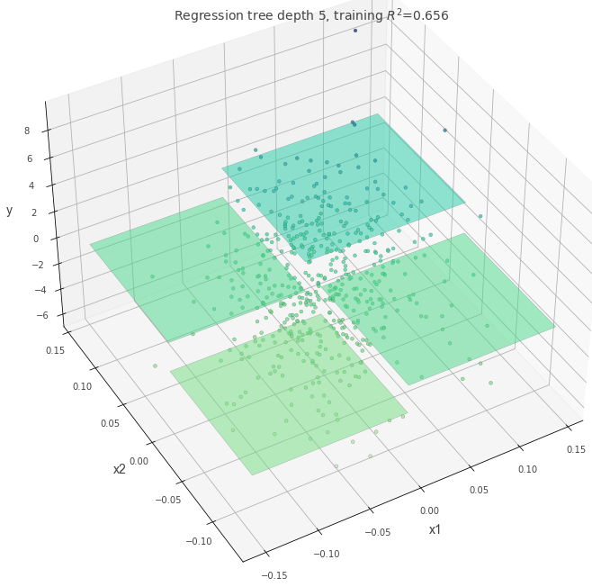
ccp_alpha=0.4

木の複雑さにペナルティを与えるパラメータです。 ccp_alphaを設定すると、値が大きいほどシンプルな木が作成されます。

dt = DecisionTreeRegressor(max_depth=5, random_state=117117, ccp_alpha=0.4)
dt.fit(X, y)

fig = plt.figure(figsize=(10, 10))
ax = fig.add_subplot(111, projection="3d")
t = rtreeviz_bivar_3D(
    dt,
    X,
    y,
    feature_names=["x1", "x2"],
    target_name="y",
    elev=40,
    azim=240,
    dist=8.0,
    show={"splits", "title"},
    ax=ax,
)
plt.show()

png

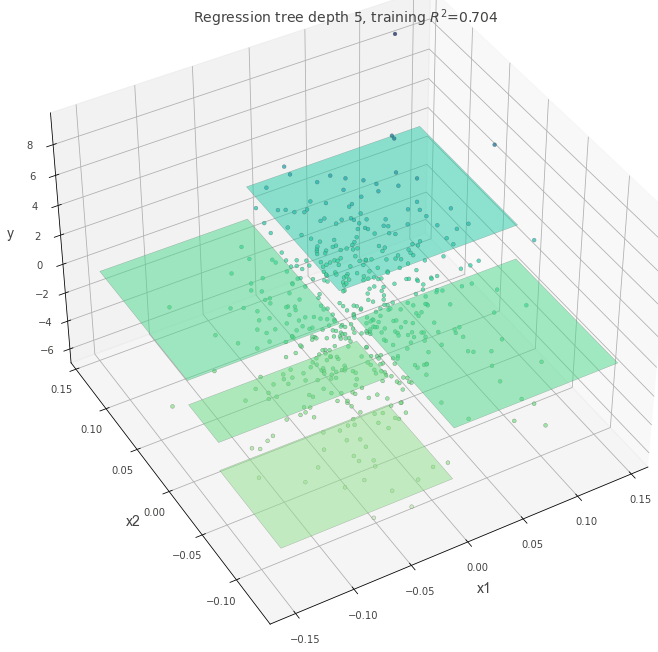
max_leaf_nodes=5

最終的に作成される葉の数を指定するパラメタです。 max_leaf_nodesの数が、区画の数と一致していることが確認できます。

dt = DecisionTreeRegressor(max_depth=5, random_state=117117, max_leaf_nodes=5)
dt.fit(X, y)

fig = plt.figure(figsize=(10, 10))
ax = fig.add_subplot(111, projection="3d")
t = rtreeviz_bivar_3D(
    dt,
    X,
    y,
    feature_names=["x1", "x2"],
    target_name="y",
    elev=40,
    azim=240,
    dist=8.0,
    show={"splits", "title"},
    ax=ax,
)
plt.show()

png

外れ値がある場合

分岐を作成する際にどの基準を適用するか指定します。外れ値がある状態で、criterion="squared_error"を指定した場合に木にどのような変化があるかを確認してみます。 absolute_error よりも squared_error の方が外れ値に強いペナルティを与えるため、squared_error と指定した場合は決定木の分岐が作成されることが予想されます。

## 外れ値として、一部のデータの値を5倍にする
X, y = make_regression(n_samples=100, n_features=2, random_state=11)
y[1:20] = y[1:20] * 5

dt = DecisionTreeRegressor(max_depth=5, random_state=117117, criterion="absolute_error")
dt.fit(X, y)

fig = plt.figure(figsize=(10, 10))
ax = fig.add_subplot(111, projection="3d")
t = rtreeviz_bivar_3D(
    dt,
    X,
    y,
    feature_names=["x1", "x2"],
    target_name="y",
    elev=40,
    azim=240,
    dist=8.0,
    show={"splits", "title"},
    ax=ax,
)
plt.show()

png

dt = DecisionTreeRegressor(max_depth=5, random_state=117117, criterion="squared_error")

dt.fit(X, y)

fig = plt.figure(figsize=(10, 10))
ax = fig.add_subplot(111, projection="3d")
t = rtreeviz_bivar_3D(
    dt,
    X,
    y,
    feature_names=["x1", "x2"],
    target_name="y",
    elev=40,
    azim=240,
    dist=8.0,
    show={"splits", "title"},
    ax=ax,
)
plt.show()

png