相互相関
import japanize_matplotlib
import numpy as np
import os
import pandas as pd
import matplotlib.pyplot as plt
import seaborn as sns
from full_fred.fred import Fred

# FRED_API_KEY = os.getenv('FRED_API_KEY')
fred = Fred()
print(f"FRED APIキーが環境変数に設定されている:{fred.env_api_key_found()}")


def get_fred_data(name, start="2013-01-01", end=""):
    df = fred.get_series_df(name)[["date", "value"]].copy()
    df["date"] = pd.to_datetime(df["date"])
    df["value"] = pd.to_numeric(df["value"], errors="coerce")
    df = df.set_index("date")

    if end == "":
        df = df.loc[f"{start}":]
    else:
        df = df.loc[f"{start}":f"{end}"]

    return df
FRED APIキーが環境変数に設定されている:True
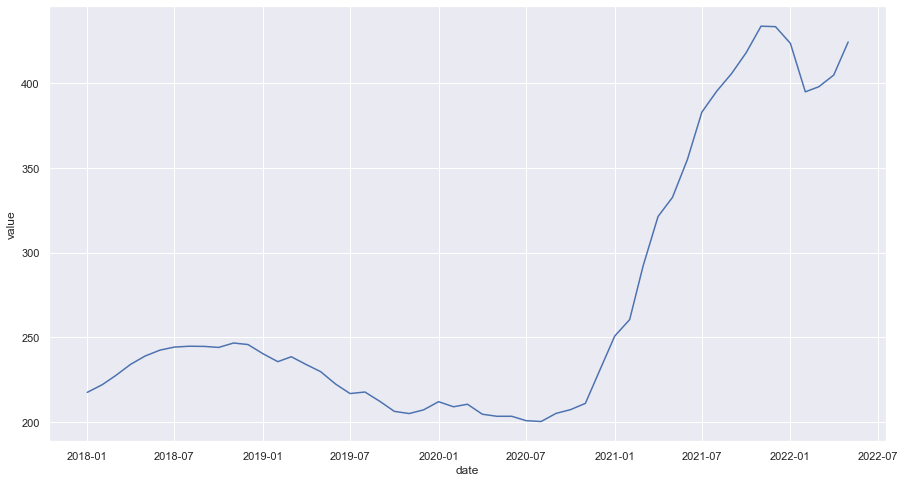
Producer Price Index by Commodity: Metals and Metal Products: Iron and Steel
ソース: https://fred.stlouisfed.org/series/WPU101
鉄及び鋼の生産者物価指数
df_WPU101 = get_fred_data("WPU101", start="2018-01-01", end="2022-05-01")
df_WPU101.head(5)
| value | |
|---|---|
| date | |
| 2018-01-01 | 217.6 |
| 2018-02-01 | 222.1 |
| 2018-03-01 | 227.5 |
| 2018-04-01 | 234.1 |
| 2018-05-01 | 239.0 |
sns.set(rc={"figure.figsize": (15, 8)})
sns.lineplot(data=df_WPU101, x="date", y="value")
<AxesSubplot:xlabel='date', ylabel='value'>
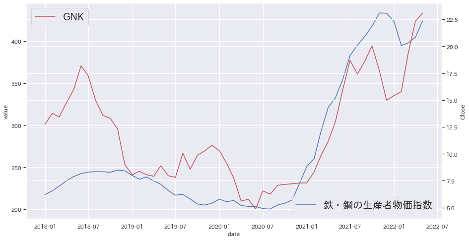
GNKの価格推移
Genco Shipping & Trading Limited ($GNK)の株価と上記グラフを比較してみます。
df_GNK = pd.read_csv("./GNK.csv")
df_GNK["Date"] = pd.to_datetime(df_GNK["Date"])
df_GNK = df_GNK.set_index("Date").resample("M").mean()
df_GNK.index = df_GNK.index + pd.DateOffset(1)  # 日付を月初に調整する
df_GNK = df_GNK.loc["2018-01-01":"2022-05-01"]
df_GNK.head()
| Open | High | Low | Close | Adj Close | Volume | |
|---|---|---|---|---|---|---|
| Date | ||||||
| 2018-01-01 | 12.5575 | 13.4355 | 12.1375 | 12.7650 | 11.157512 | 603175.0 |
| 2018-02-01 | 13.9720 | 14.5420 | 13.1310 | 13.7600 | 12.027212 | 510600.0 |
| 2018-03-01 | 12.9925 | 13.8525 | 12.6520 | 13.4300 | 11.738769 | 357050.0 |
| 2018-04-01 | 15.0100 | 15.6925 | 14.4025 | 14.7575 | 12.899099 | 796075.0 |
| 2018-05-01 | 15.5280 | 16.3530 | 14.9620 | 15.9580 | 13.948420 | 631500.0 |
japanize_matplotlib.japanize()

fig = plt.figure()
ax1 = fig.add_subplot(111)
sns.lineplot(data=df_WPU101, x="date", y="value", label="鉄・鋼の生産者物価指数")
plt.legend(loc="lower right", fontsize="20")

ax2 = ax1.twinx()
sns.lineplot(data=df_GNK, x="Date", y="Close", label="GNK", color="r")
plt.legend(loc="upper left", fontsize="20")
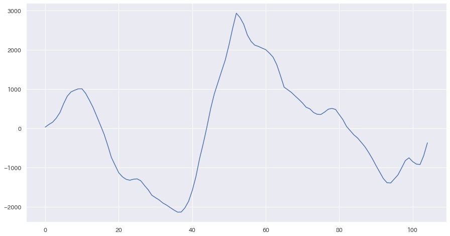
相互相関を求める
相互相関関数は、ふたつの信号、配列(ベクトル)の類似性を確認するために使われる。関数の配列の結果がすべて1であれば相関があり、すべてゼロであれば無相関であり、すべて −1 であれば負の相関がある。しばしば、相関と略されることがあり、相関係数と似ているために混同することがある。 (出典:Wikipedia)
ドキュメント: numpy.correlate
df_GNK["Close_norm"] = df_GNK["Close"] - df_GNK["Close"].mean()
df_WPU101["value_norm"] = df_WPU101["value"] - df_WPU101["value"].mean()

corr = np.correlate(df_GNK["Close_norm"], df_WPU101["value_norm"], "full")
delay = corr.argmax() - (len(df_WPU101["value_norm"]) - 1)
print("ラグ: " + str(delay))

plt.plot(corr)
ラグ: 0


[<matplotlib.lines.Line2D at 0x13e252170>]
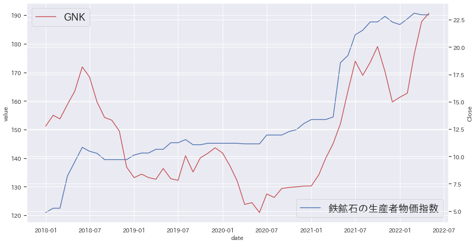
Producer Price Index by Industry: Iron Ore Mining
ソース:https://fred.stlouisfed.org/series/PCU2122121221
鉄鉱石の生産者物価指数
df_PCU2122121221 = get_fred_data("PCU2122121221", start="2018-01-01", end="2022-05-01")
df_PCU2122121221.head(5)
| value | |
|---|---|
| date | |
| 2018-01-01 | 121.0 |
| 2018-02-01 | 122.5 |
| 2018-03-01 | 122.5 |
| 2018-04-01 | 133.8 |
| 2018-05-01 | 138.7 |
fig = plt.figure()
ax1 = fig.add_subplot(111)
sns.lineplot(data=df_PCU2122121221, x="date", y="value", label="鉄鉱石の生産者物価指数")
plt.legend(loc="lower right", fontsize="20")

ax2 = ax1.twinx()
sns.lineplot(data=df_GNK, x="Date", y="Close", label="GNK", color="r")
plt.legend(loc="upper left", fontsize="20")
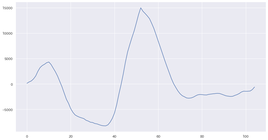
df_PCU2122121221["value_norm"] = (
    df_PCU2122121221["value"] - df_PCU2122121221["value"].mean()
)

corr = np.correlate(df_GNK["Close_norm"], df_PCU2122121221["value_norm"], "full")
delay = corr.argmax() - (len(df_PCU2122121221["value_norm"]) - 1)
print("ラグ: " + str(delay))

plt.plot(corr)
ラグ: 0


[<matplotlib.lines.Line2D at 0x13e373fa0>]