Prophetのパラメータ

Prophetにどのようなパラメータがあるか整理します。

import numpy as np
import pandas as pd
import seaborn as sns
import matplotlib.pyplot as plt
import japanize_matplotlib
from prophet import Prophet

実験に使用するデータ

date = pd.date_range("2020-01-01", periods=365, freq="D")

# 予測対象
y = [
    np.cos(di.weekday()) / 3
    + di.month % 2 / 5
    + np.log(i + 1) / 5.0
    + (i > 182) * 0.5
    + np.random.rand() / 10
    for i, di in enumerate(date)
]

# トレンド成分
x = [18627 + i - 364 for i in range(365)]
trend_y = [np.log(i + 1) / 3.0 for i, di in enumerate(date)]
weekly_y = [np.cos(di.weekday()) for i, di in enumerate(date)]
seasonal_y = [di.month % 2 / 2 for i, di in enumerate(date)]
noise_y = [np.random.rand() / 10 for i in range(365)]

df = pd.DataFrame({"ds": date, "y": y})
df.index = date

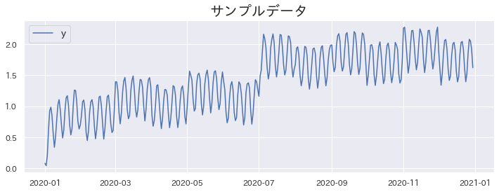
# 実験に使用するデータ
plt.title("サンプルデータ")
sns.lineplot(data=df)
plt.show()

growthパラメータ

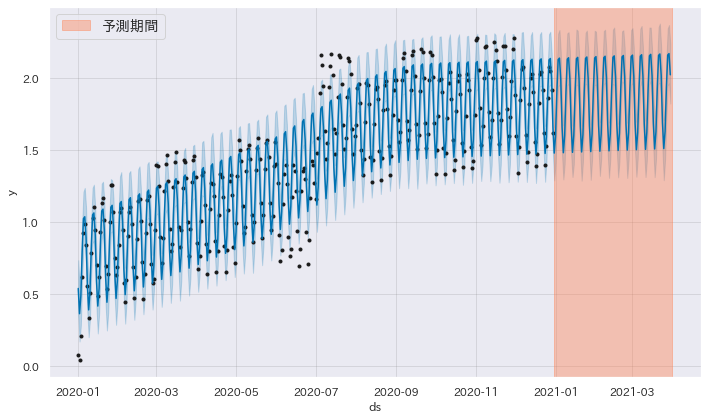
growth=“linear"とした場合の予測

# モデルを訓練
m = Prophet(
    yearly_seasonality=False,
    weekly_seasonality=True,
    daily_seasonality=False,
    growth="linear",
)
m.fit(df)

# 将来を予測
future = m.make_future_dataframe(periods=90)
forecast = m.predict(future)
fig = m.plot(forecast)
plt.axvspan(18627, 18627 + 90, color="coral", alpha=0.4, label="予測期間")
plt.legend()
plt.show()

Initial log joint probability = -16.6231
    Iter      log prob        ||dx||      ||grad||       alpha      alpha0  # evals  Notes 
      81       792.152    0.00138864       97.2266   2.443e-05       0.001      145  LS failed, Hessian reset 
      99       792.228   7.40168e-07       55.8404     0.03797     0.03797      168   
    Iter      log prob        ||dx||      ||grad||       alpha      alpha0  # evals  Notes 
     138       792.388   3.51776e-05       59.7965    6.64e-07       0.001      263  LS failed, Hessian reset 
     199        792.62    3.0252e-05       72.8985      0.4243           1      340   
    Iter      log prob        ||dx||      ||grad||       alpha      alpha0  # evals  Notes 
     247       792.799   0.000165183       55.2724   3.174e-06       0.001      440  LS failed, Hessian reset 
     299       792.972   0.000162358       62.7075           1           1      508   
    Iter      log prob        ||dx||      ||grad||       alpha      alpha0  # evals  Notes 
     347       792.991   3.19534e-05       38.7196   4.536e-07       0.001      634  LS failed, Hessian reset 
     392       792.994   7.68689e-07       61.3331   1.015e-08       0.001      733  LS failed, Hessian reset 
     399       792.994     9.628e-08       55.3164      0.2134           1      742   
    Iter      log prob        ||dx||      ||grad||       alpha      alpha0  # evals  Notes 
     404       792.994   3.74603e-08       39.3307      0.2405      0.7727      749   
Optimization terminated normally: 
  Convergence detected: relative gradient magnitude is below tolerance

growth=“linear"で表現できるトレンド成分

growth=“linear"でどのようなトレンドを表現できるか確認してみます。 linear_trend はprophetで growth="linear"　を指定した時にトレンド作成に使用するコードを再現してみます。

※参考文献のコードと記号を合わせました、ミスがある場合はお手数ですがissueに指摘いただけると大変助かります

$A$の各行の次元数は変化点の数です。また、各次元の値は $ a_j(t) \left{ \begin{array}{ll} 1, & \text{if}　\ t \ge s_j \ 0, & \text{otherwise} \end{array} \right. $ となっています。時刻$t$の$a$の$j$次元目は、$t$が$j$番目の変化点よりあとの時刻ならば$1$になる、ということです。

def linear_trend(
    k: float, m: float, delta: np.array, t: np.array, t_change: list
) -> np.array:
    """線形トレンドを作成する

    Args:
        k (float): 係数
        m (float): 係数
        delta (np.array): delta
        t (np.array): タイムスタンプ
        t_change (list): トレンド変化点

    Returns:
        np.array: トレンド
    """
    A = np.vstack([np.where(t_change < ti, 1, 0) for ti in t])
    return (k + (A * delta).sum(axis=1)) * t + (
        m + (A * (-t_change * delta)).sum(axis=1)
    )

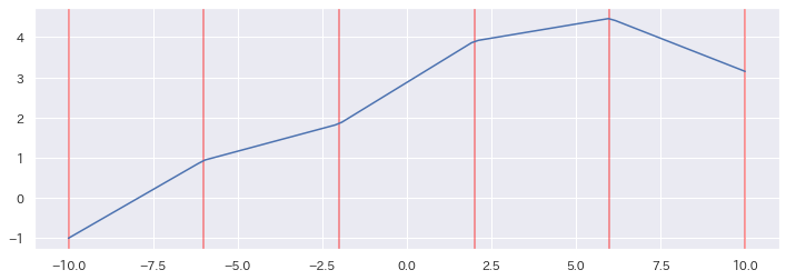
linear_trendで表現できるトレンドを可視化する

# 適当にトレンドのような線を作成するため、変化点の数と各区間での線の傾きを指定します
change_point_num = 5
t = np.linspace(-10, 10, 100)
t_change = np.linspace(-10, 10, change_point_num + 1)
delta = np.array([np.random.rand() - 0.5 for _ in range(change_point_num + 1)])

# linear_trendで線を引く
trend_y = linear_trend(0.1, 0, delta, t, t_change)

# できた線をプロットしてみる
[plt.axvline(x=tci, color="red", alpha=0.5) for tci in t_change]  # 変化点をプロット
plt.plot(t, trend_y)
plt.show()