Isolation Forest で異常点を検知する

直感 #

部屋に 1,000 人が集まっていて、1 人だけ隅に離れて立っているとします。部屋をランダムな位置の仕切りで何回も区切ると、隅の 1 人は 2〜3 回で「仕切りの中に自分しかいない」状態になります。一方、人混みの中の 1 人を孤立させるには 10 回以上仕切る必要があります。Isolation Forest はこの「孤立するまでの分割回数（経路長）」を木ごとに記録し、200 本の木で平均した経路長が短い点ほど異常スコアを高くします。分割の軸も位置もランダムなので、データが三日月形でもリング形でも、密集地から離れた点を同じ理屈で拾えます。

データの準備 #

次のコードは三日月形 2 つに並んだ 1,000 点を作り、60 点ごとに 1 点、計 17 点の座標を 2.5 倍に引き伸ばして外れ点にします。正解の位置が分かっているので、検知結果の赤丸がこの × と重なるかで性能を確認できます。

 1
 2
 3
 4
 5
 6
 7
 8
 9
10
11
12
13
14
15
16
17

import numpy as np
import matplotlib.pyplot as plt
from sklearn.datasets import make_moons

rng = np.random.default_rng(42)
X, _ = make_moons(n_samples=1_000, noise=0.08, random_state=42)

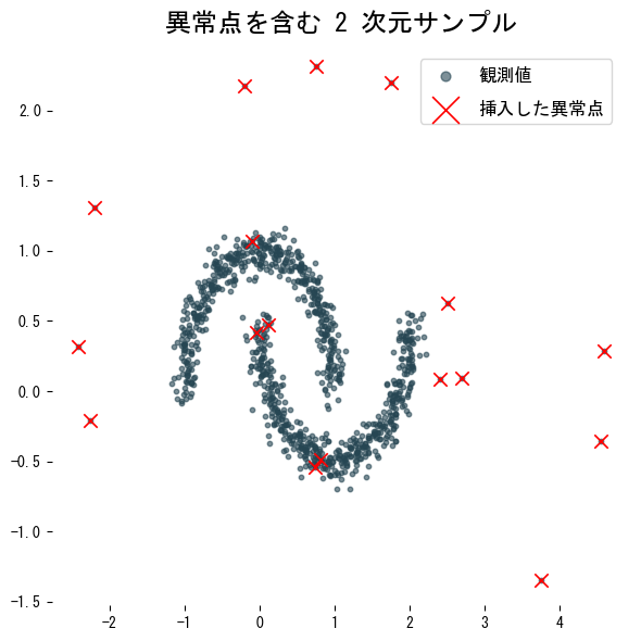
anomaly_index = np.arange(0, 1_000, 60)
X[anomaly_index] *= 2.5  # 一部サンプルを拡大して外れ点にする

plt.figure(figsize=(6, 6))
plt.scatter(X[:, 0], X[:, 1], s=10, alpha=0.6, label="観測値")
plt.scatter(X[anomaly_index, 0], X[anomaly_index, 1], marker="x", s=80, c="red", label="挿入した異常点")
plt.legend()
plt.title("異常点を含む 2 次元サンプル")
plt.tight_layout()
plt.show()

何が起きているか（ステップで見る） #

コードを読む前に、この手法が図の上で何をしているかを追ってみましょう。「再生」を押すか、スライダーを動かすと 1 手順ずつ進みます。

見るポイント：少ない回数で孤立する点ほど異常。外れ値（赤）は 1〜5 回の分割で 1 点だけになり、密集した点（青）は 8 回切っても 5 点が残る。

Isolation Forest で学習・検知 #

次のコードは 200 本の木を作って各点の経路長を平均し、スコアの低い下位 2% に −1（異常）のラベルを付けます。

 1
 2
 3
 4
 5
 6
 7
 8
 9
10
11
12
13

from sklearn.ensemble import IsolationForest

detector = IsolationForest(
    n_estimators=200,
    max_samples=256,
    contamination=0.02,
    random_state=42,
)
detector.fit(X)

scores = detector.decision_function(X)
pred = detector.predict(X)  # -1: outlier, 1: inlier
detected_index = np.where(pred < 0)[0]

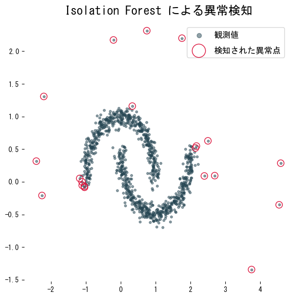
contamination はデータ中の異常比率の上限を指定するパラメーターで、比率が不明な場合は 0.01 程度の小さめの値から始めて、検知された点を目で確かめながら上げていくと安定します。

結果を可視化する #

次のコードは predict が −1 を返した点を赤い丸で囲み、最初の図の × と重なるかを確かめます。

 1
 2
 3
 4
 5
 6
 7
 8
 9
10
11
12
13
14

plt.figure(figsize=(6, 6))
plt.scatter(X[:, 0], X[:, 1], s=10, alpha=0.5, label="観測値")
plt.scatter(
    X[detected_index, 0],
    X[detected_index, 1],
    facecolor="none",
    edgecolor="crimson",
    s=90,
    label="検知された異常点",
)
plt.title("Isolation Forest による異常検知")
plt.legend()
plt.tight_layout()
plt.show()

実行結果の読み方 #

赤い丸は三日月の外に飛び出した 17 点の × をほぼすべて囲み、残りの数個は三日月の先端など密度が薄い場所に付きます。contamination=0.02 は 20 点を異常と呼ぶ設定なので、正解 17 点との差 3 点が誤検知として現れるのは仕様どおりです。scores を見ると、× の点は大きく負の値、三日月の先端の誤検知は 0 に近い値になっているので、閾値を少し下げるだけで切り分けられます。

使いどころと落とし穴 #

contamination を大きくしすぎると正常値まで異常判定されやすくなるので、監視ログなどでは 0.01 以下から試すのが無難です。max_samples は 256 が初期値としてよく使われ、データ量が多い場合に値を増やすと決定境界が滑らかになります。後からしきい値を変えたいときは decision_function のスコアを保存しておき、predict の −1/1 ラベルは最終判定にだけ使います。特徴量ごとにスケールが大きく異なる場合は、分割点がランダムとはいえ範囲の広い軸ばかりが選ばれやすくなるので、StandardScaler や RobustScaler で揃えてから渡すと検知性能が安定します。