Modelos de Mistura Gaussiana (GMM)

Atualizado 2020-03-25 Leitura 3 min

Resumo

Um Modelo de Mistura Gaussiana representa os dados como uma soma ponderada de componentes normais multivariadas.
Ele produz uma matriz de responsabilidades que quantifica o quanto cada componente explica cada amostra.
Os parâmetros são estimados com o algoritmo EM; as estruturas de covariância podem ser full, tied, diag ou spherical.
A seleção de modelo tipicamente combina critérios de informação (BIC/AIC) com múltiplas inicializações aleatórias para estabilidade.

Intuição #

Este método deve ser interpretado por meio de suas suposições, condições dos dados e como as escolhas de parâmetros afetam a generalização.

Explicação Detalhada #

Formulação Matemática #

A densidade de $\mathbf{x}$ é

$$ p(\mathbf{x}) = \sum_{k=1}^{K} \pi_k \, \mathcal{N}(\mathbf{x} \mid \boldsymbol{\mu}_k, \boldsymbol{\Sigma}_k), $$

com pesos de mistura $\pi_k$ (não negativos e com soma igual a 1). O EM alterna:

Etapa E: calcular responsabilidades $\gamma_{ik}$. $$ \gamma_{ik} = \frac{\pi_k \, \mathcal{N}(\mathbf{x}_i \mid \boldsymbol{\mu}_k, \boldsymbol{\Sigma}_k)} {\sum_{j=1}^K \pi_j \, \mathcal{N}(\mathbf{x}_i \mid \boldsymbol{\mu}_j, \boldsymbol{\Sigma}_j)}. $$
Etapa M: re-estimar $\pi_k, \boldsymbol{\mu}_k, \boldsymbol{\Sigma}k$ usando $\gamma{ik}$ como pesos.

A log-verossimilhança aumenta monotonicamente e converge para um ótimo local.

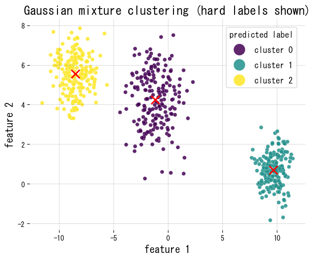
Experimentos em Python #

Ajustamos um GMM a blobs sintéticos em 2D, plotamos as atribuições rígidas e reportamos os pesos de mistura e o formato da matriz de responsabilidades.

from __future__ import annotations

import matplotlib.pyplot as plt
import numpy as np
from numpy.typing import NDArray
from sklearn.datasets import make_blobs
from sklearn.mixture import GaussianMixture

def run_gmm_demo(
    n_samples: int = 600,
    n_components: int = 3,
    cluster_std: list[float] | tuple[float, ...] = (1.0, 1.4, 0.8),
    covariance_type: str = "full",
    random_state: int = 7,
    n_init: int = 8,
) -> dict[str, object]:
    """Fit a Gaussian mixture model and visualise hard labels with component centres."""
    features, _ = make_blobs(
        n_samples=n_samples,
        centers=n_components,
        cluster_std=cluster_std,
        random_state=random_state,
    )

    gmm = GaussianMixture(
        n_components=n_components,
        covariance_type=covariance_type,
        random_state=random_state,
        n_init=n_init,
    )
    gmm.fit(features)

    hard_labels = gmm.predict(features)
    responsibilities = gmm.predict_proba(features)
    log_likelihood = float(gmm.score(features))
    weights = gmm.weights_

    fig, ax = plt.subplots(figsize=(6.2, 5.2))
    scatter = ax.scatter(
        features[:, 0],
        features[:, 1],
        c=hard_labels,
        cmap="viridis",
        s=30,
        edgecolor="white",
        linewidth=0.2,
        alpha=0.85,
    )
    ax.scatter(
        gmm.means_[:, 0],
        gmm.means_[:, 1],
        marker="x",
        c="red",
        s=140,
        linewidth=2.0,
        label="Component centre",
    )
    ax.set_title("Gaussian mixture clustering (hard labels shown)")
    ax.set_xlabel("feature 1")
    ax.set_ylabel("feature 2")
    ax.grid(alpha=0.2)
    handles, _ = scatter.legend_elements()
    labels = [f"cluster {idx}" for idx in range(n_components)]
    ax.legend(handles, labels, title="predicted label", loc="upper right")
    fig.tight_layout()
    plt.show()

    return {
        "log_likelihood": log_likelihood,
        "weights": weights.tolist(),
        "responsibilities_shape": responsibilities.shape,
    }

metrics = run_gmm_demo()
print(f"log-likelihood: {metrics['log_likelihood']:.3f}")
print("mixture weights:", metrics["weights"])
print("responsibility matrix shape:", metrics["responsibilities_shape"])

Ajustamos um GMM a blobs sintéticos em 2D, plotamos a atribuição rígida… figura

Referências #

Bishop, C. M. (2006). Pattern Recognition and Machine Learning. Springer.
Dempster, A. P., Laird, N. M., & Rubin, D. B. (1977). Maximum Likelihood from Incomplete Data via the EM Algorithm. Journal of the Royal Statistical Society, Series B.
scikit-learn developers. (2024). Gaussian Mixture Models. https://scikit-learn.org/stable/modules/mixture.html