2.4.4
Adaboost (Regressão)
Resumo- A regressão AdaBoost (AdaBoost.R2) melhora as previsões reponderando amostras com maiores erros residuais.
- As atualizações de pesos dependem do perfil de erro, então ruído e outliers afetam diretamente o conjunto final.
- A validação cruzada de
n_estimators e learning_rate é essencial para equilibrar a qualidade do ajuste e a generalização.
Intuição
#
A regressão AdaBoost enfatiza repetidamente as regiões onde os preditores atuais têm desempenho fraco. Ao realocar a atenção para amostras com alto erro, o conjunto captura padrões residuais não lineares que aprendizes individuais frequentemente ignoram.
Explicação Detalhada
#
1
2
3
4
5
| import numpy as np
import matplotlib.pyplot as plt
import japanize_matplotlib
from sklearn.tree import DecisionTreeRegressor
from sklearn.ensemble import AdaBoostRegressor
|
 1
 2
 3
 4
 5
 6
 7
 8
 9
10
11
12
13
14
15
16
17
18
19
20
21
22
23
24
25
26
27
| # NOTA: Este modelo serve para verificar o sample_weight do modelo
class DummyRegressor:
def __init__(self):
self.model = DecisionTreeRegressor(max_depth=5)
self.error_vector = None
self.X_for_plot = None
self.y_for_plot = None
def fit(self, X, y):
self.model.fit(X, y)
y_pred = self.model.predict(X)
# Os pesos são calculados com base no erro de regressão.
# https://github.com/scikit-learn/scikit-learn/blob/main/sklearn/ensemble/_weight_boosting.py#L1130
self.error_vector = np.abs(y_pred - y)
self.X_for_plot = X.copy()
self.y_for_plot = y.copy()
return self.model
def predict(self, X, check_input=True):
return self.model.predict(X)
def get_params(self, deep=False):
return {}
def set_params(self, deep=False):
return {}
|
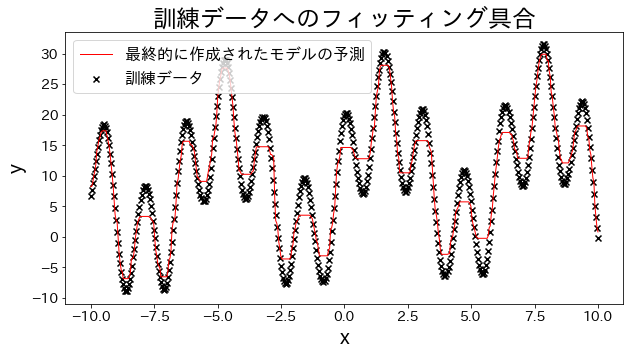
Ajustar modelos de regressão aos dados de treinamento
#
 1
 2
 3
 4
 5
 6
 7
 8
 9
10
11
12
13
14
15
16
17
18
19
20
21
22
23
| # training dataset
X = np.linspace(-10, 10, 500)[:, np.newaxis]
y = (np.sin(X).ravel() + np.cos(4 * X).ravel()) * 10 + 10 + np.linspace(-2, 2, 500)
## train Adaboost regressor
reg = AdaBoostRegressor(
DummyRegressor(),
n_estimators=100,
random_state=100,
loss="linear",
learning_rate=0.8,
)
reg.fit(X, y)
y_pred = reg.predict(X)
# Verificar o ajuste aos dados de treinamento.
plt.figure(figsize=(10, 5))
plt.scatter(X, y, c="k", marker="x", label="訓練データ")
plt.plot(X, y_pred, c="r", label="prediction", linewidth=1)
plt.xlabel("x")
plt.ylabel("y")
plt.legend()
plt.show()
|
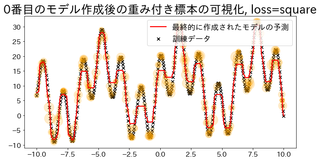
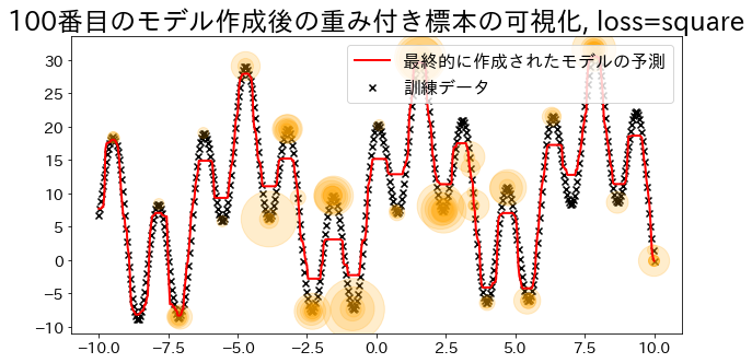
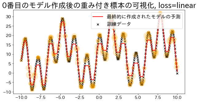
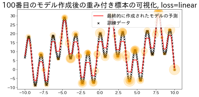
Visualizar pesos das amostras (para loss=‘linear’)
#
O Adaboost determina os pesos com base nos erros da regressão. Visualize a magnitude dos pesos quando especificado como ’linear’. Observe como os dados com pesos adicionados têm maior probabilidade de serem amostrados durante o treinamento.
loss{’linear’, ‘square’, ’exponential’}, default=‘linear’
The loss function to use when updating the weights after each boosting iteration.
 1
 2
 3
 4
 5
 6
 7
 8
 9
10
11
12
13
14
15
16
17
18
19
20
21
22
23
24
25
26
27
28
29
30
31
32
33
34
35
36
37
38
39
40
41
42
43
44
45
46
47
48
49
50
51
52
53
54
| def visualize_weight(reg, X, y, y_pred):
"""Function for plotting the value (number of times sampled) corresponding to the weights of the sample
Parameters
----------
reg : sklearn.ensemble._weight_boosting
boosting model
X : numpy.ndarray
training dataset
y : numpy.ndarray
target
y_pred:
prediction
"""
assert reg.estimators_ is not None, "len(reg.estimators_) > 0"
for i, estimators_i in enumerate(reg.estimators_):
if i % 100 == 0:
# Contar quantas vezes os dados aparecem no conjunto usado para criar o i-ésimo modelo
weight_dict = {xi: 0 for xi in X.ravel()}
for xi in estimators_i.X_for_plot.ravel():
weight_dict[xi] += 1
# Plotar o número de ocorrências como círculos laranja no gráfico (quanto maior o número, maior o círculo)
weight_x_sorted = sorted(weight_dict.items(), key=lambda x: x[0])
weight_vec = np.array([s * 100 for xi, s in weight_x_sorted])
# plot graph
plt.figure(figsize=(10, 5))
plt.title(f"Visualization of the weighted sample after creating the {i}-th model, loss={reg.loss}")
plt.scatter(X, y, c="k", marker="x", label="training data")
plt.scatter(
estimators_i.X_for_plot,
estimators_i.y_for_plot,
marker="o",
alpha=0.2,
c="orange",
s=weight_vec,
)
plt.plot(X, y_pred, c="r", label="prediction", linewidth=2)
plt.legend(loc="upper right")
plt.show()
## Criar modelo de regressão com loss="linear"
reg = AdaBoostRegressor(
DummyRegressor(),
n_estimators=101,
random_state=100,
loss="linear",
learning_rate=1,
)
reg.fit(X, y)
y_pred = reg.predict(X)
visualize_weight(reg, X, y, y_pred)
|
 1
 2
 3
 4
 5
 6
 7
 8
 9
10
11
| ## Criar modelo de regressão com loss="square"
reg = AdaBoostRegressor(
DummyRegressor(),
n_estimators=101,
random_state=100,
loss="square",
learning_rate=1,
)
reg.fit(X, y)
y_pred = reg.predict(X)
visualize_weight(reg, X, y, y_pred)
|