Resumo- O Gradient Boosting constrói um modelo aditivo ajustando cada novo aprendiz fraco ao sinal residual atual.
learning_rate e n_estimators controlam conjuntamente a velocidade de otimização e o risco de sobreajuste.- A escolha da função de perda altera a robustez a outliers e a forma da função ajustada.
Intuição
#
O Gradient Boosting começa com uma previsão aproximada, e então adiciona repetidamente pequenas árvores que corrigem o que o modelo atual ainda erra. Muitas correções pequenas e direcionadas se acumulam em um preditor flexível.
Explicação Detalhada
#
1
2
3
4
| import numpy as np
import matplotlib.pyplot as plt
import japanize_matplotlib
from sklearn.ensemble import GradientBoostingRegressor
|
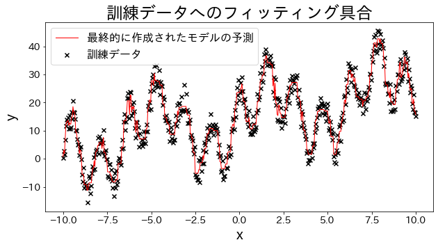
Ajustar modelo de regressão aos dados de treinamento
#
Criar dados experimentais, dados de forma de onda com funções trigonométricas somadas.
 1
 2
 3
 4
 5
 6
 7
 8
 9
10
11
12
13
14
15
16
17
18
19
20
21
22
23
24
25
26
27
28
29
| # training dataset
X = np.linspace(-10, 10, 500)[:, np.newaxis]
noise = np.random.rand(X.shape[0]) * 10
# target
y = (
(np.sin(X).ravel() + np.cos(4 * X).ravel()) * 10
+ 10
+ np.linspace(-10, 10, 500)
+ noise
)
# train gradient boosting
reg = GradientBoostingRegressor(
n_estimators=50,
learning_rate=0.5,
)
reg.fit(X, y)
y_pred = reg.predict(X)
# Verificar o ajuste aos dados de treinamento
plt.figure(figsize=(10, 5))
plt.scatter(X, y, c="k", marker="x", label="training data")
plt.plot(X, y_pred, c="r", label="Predictions for the final created model", linewidth=1)
plt.xlabel("x")
plt.ylabel("y")
plt.title("Degree of fitting to training dataset")
plt.legend()
plt.show()
|
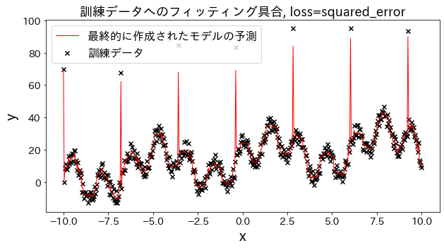
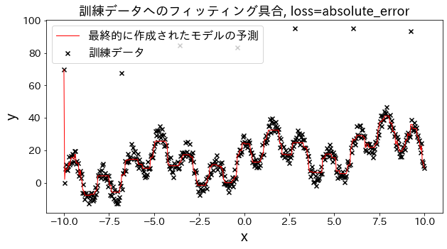
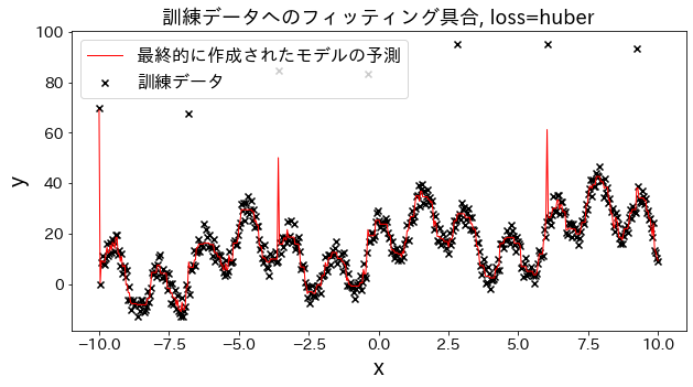
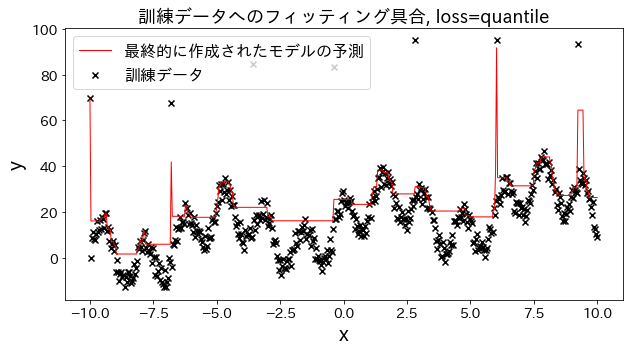
Efeito da função de perda nos resultados
#
Verifique como o ajuste aos dados de treinamento muda quando a perda é alterada para [“squared_error”, “absolute_error”, “huber”, “quantile”]. Espera-se que “absolute_error” e “huber” não prossigam para prever outliers, já que a penalidade para outliers não é tão grande quanto o erro quadrático.
 1
 2
 3
 4
 5
 6
 7
 8
 9
10
11
12
13
14
15
16
17
18
19
20
21
22
23
24
25
26
27
28
29
30
31
32
33
34
35
36
| # training data
X = np.linspace(-10, 10, 500)[:, np.newaxis]
# prepare outliers
noise = np.random.rand(X.shape[0]) * 10
for i, ni in enumerate(noise):
if i % 80 == 0:
noise[i] = 70 + np.random.randint(-10, 10)
# target
y = (
(np.sin(X).ravel() + np.cos(4 * X).ravel()) * 10
+ 10
+ np.linspace(-10, 10, 500)
+ noise
)
for loss in ["squared_error", "absolute_error", "huber", "quantile"]:
# train gradient boosting
reg = GradientBoostingRegressor(
n_estimators=50,
learning_rate=0.5,
loss=loss,
)
reg.fit(X, y)
y_pred = reg.predict(X)
# Verificar o ajuste aos dados de treinamento.
plt.figure(figsize=(10, 5))
plt.scatter(X, y, c="k", marker="x", label="training dataset")
plt.plot(X, y_pred, c="r", label="Predictions for the final created model", linewidth=1)
plt.xlabel("x")
plt.ylabel("y")
plt.title(f"Degree of fitting to training data, loss={loss}", fontsize=18)
plt.legend()
plt.show()
|
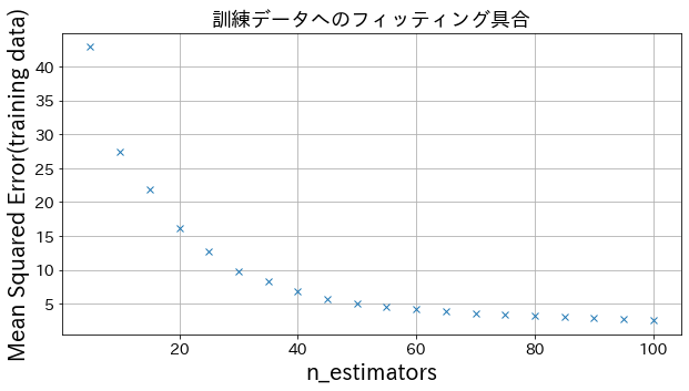
Efeito do n_estimators nos resultados
#
Você pode ver como o grau de melhoria atinge um ponto de saturação quando aumenta o n_estimators até certo ponto.
 1
 2
 3
 4
 5
 6
 7
 8
 9
10
11
12
13
14
15
16
17
18
19
20
21
22
23
24
25
26
27
28
29
30
31
32
33
| from sklearn.metrics import mean_squared_error as MSE
# trainig dataset
X = np.linspace(-10, 10, 500)[:, np.newaxis]
noise = np.random.rand(X.shape[0]) * 10
# target
y = (
(np.sin(X).ravel() + np.cos(4 * X).ravel()) * 10
+ 10
+ np.linspace(-10, 10, 500)
+ noise
)
# Tentar criar um modelo com diferentes n_estimators
n_estimators_list = [(i + 1) * 5 for i in range(20)]
mses = []
for n_estimators in n_estimators_list:
reg = GradientBoostingRegressor(
n_estimators=n_estimators,
learning_rate=0.3,
)
reg.fit(X, y)
y_pred = reg.predict(X)
mses.append(MSE(y, y_pred))
# Plotar mean_squared_error para diferentes n_estimators
plt.figure(figsize=(10, 5))
plt.plot(n_estimators_list, mses, "x")
plt.xlabel("n_estimators")
plt.ylabel("Mean Squared Error(training data)")
plt.grid()
plt.show()
|
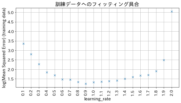
Impacto do learning_rate nos resultados
#
Se o learning_rate for muito pequeno, a precisão não melhora, e se o learning_rate for muito grande, não converge.
 1
 2
 3
 4
 5
 6
 7
 8
 9
10
11
12
13
14
15
16
17
18
19
20
21
| # Tentar criar um modelo com diferentes n_estimators
learning_rate_list = [np.round(0.1 * (i + 1), 1) for i in range(20)]
mses = []
for learning_rate in learning_rate_list:
reg = GradientBoostingRegressor(
n_estimators=30,
learning_rate=learning_rate,
)
reg.fit(X, y)
y_pred = reg.predict(X)
mses.append(np.log(MSE(y, y_pred)))
# Plotar mean_squared_error para diferentes n_estimators
plt.figure(figsize=(10, 5))
plt_index = [i for i in range(len(learning_rate_list))]
plt.plot(plt_index, mses, "x")
plt.xticks(plt_index, learning_rate_list, rotation=90)
plt.xlabel("learning_rate", fontsize=15)
plt.ylabel("log(Mean Squared Error) (training data)", fontsize=15)
plt.grid()
plt.show()
|