2.1.11
Mínimos Quadrados Ponderados (WLS)
Resumo
- Os Mínimos Quadrados Ponderados atribuem pesos específicos por observação para que medições confiáveis influenciem mais fortemente a reta ajustada.
- Multiplicar os erros quadrados por pesos reduz a importância de observações com alta variância e mantém a estimativa próxima dos dados confiáveis.
- Você pode executar WLS com a
LinearRegressiondo scikit-learn fornecendosample_weight. - Os pesos podem vir de variâncias conhecidas, diagnósticos de resíduos ou conhecimento de domínio; o design cuidadoso é crucial.
Intuição #
Este método deve ser interpretado através de suas suposições, condições dos dados e como as escolhas de parâmetros afetam a generalização.
Explicação Detalhada #
Formulação Matemática #
Com pesos positivos \(w_i\), minimize
$$ L(\boldsymbol\beta, b) = \sum_{i=1}^{n} w_i \left(y_i - (\boldsymbol\beta^\top \mathbf{x}_i + b)\right)^2. $$A escolha ótima \(w_i \propto 1/\sigma_i^2\) (variância inversa) dá mais influência às observações precisas.
Experimentos em Python #
Comparamos OLS e WLS em dados cujo nível de ruído difere entre regiões.
from __future__ import annotations
import japanize_matplotlib
import matplotlib.pyplot as plt
import numpy as np
from sklearn.linear_model import LinearRegression
def run_weighted_vs_ols(
n_samples: int = 200,
threshold: float = 5.0,
low_noise: float = 0.5,
high_noise: float = 2.5,
xlabel: str = "input $",
ylabel: str = "output $",
label_scatter: str = "observations (color=noise)",
label_truth: str = "true line",
label_ols: str = "OLS",
label_wls: str = "WLS",
title: str | None = None,
) -> dict[str, float]:
"""Compare OLS and weighted least squares on heteroscedastic data.
Args:
n_samples: Number of evenly spaced samples to generate.
threshold: Breakpoint separating low- and high-noise regions.
low_noise: Noise scale for the lower region.
high_noise: Noise scale for the higher region.
xlabel: Label for the x-axis.
ylabel: Label for the y-axis.
label_scatter: Legend label for the colored scatter plot.
label_truth: Legend label for the ground-truth line.
label_ols: Legend label for the OLS fit.
label_wls: Legend label for the WLS fit.
title: Optional title for the plot.
Returns:
Dictionary with slopes and intercepts of both fits.
"""
japanize_matplotlib.japanize()
rng = np.random.default_rng(7)
X_vals: np.ndarray = np.linspace(0.0, 10.0, n_samples, dtype=float)
true_y: np.ndarray = 1.2 * X_vals + 3.0
noise_scale = np.where(X_vals < threshold, low_noise, high_noise)
y_noisy = true_y + rng.normal(scale=noise_scale)
weights = 1.0 / (noise_scale**2)
X = X_vals[:, np.newaxis]
ols = LinearRegression()
ols.fit(X, y_noisy)
wls = LinearRegression()
wls.fit(X, y_noisy, sample_weight=weights)
grid = np.linspace(0.0, 10.0, 200, dtype=float)[:, np.newaxis]
ols_pred = ols.predict(grid)
wls_pred = wls.predict(grid)
fig, ax = plt.subplots(figsize=(10, 5))
scatter = ax.scatter(
X,
y_noisy,
c=noise_scale,
cmap="coolwarm",
s=25,
label=label_scatter,
)
ax.plot(grid, 1.2 * grid.ravel() + 3.0, color="#2ca02c", label=label_truth)
ax.plot(grid, ols_pred, color="#1f77b4", linestyle="--", linewidth=2, label=label_ols)
ax.plot(grid, wls_pred, color="#d62728", linewidth=2, label=label_wls)
ax.set_xlabel(xlabel)
ax.set_ylabel(ylabel)
if title:
ax.set_title(title)
ax.legend()
fig.tight_layout()
plt.show()
return {
"ols_slope": float(ols.coef_[0]),
"ols_intercept": float(ols.intercept_),
"wls_slope": float(wls.coef_[0]),
"wls_intercept": float(wls.intercept_),
}
metrics = run_weighted_vs_ols()
print(f"OLS slope: {metrics['ols_slope']:.3f}, intercept: {metrics['ols_intercept']:.3f}")
print(f"WLS slope: {metrics['wls_slope']:.3f}, intercept: {metrics['wls_intercept']:.3f}")

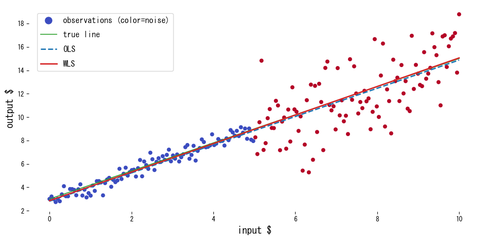
Interpretação dos resultados #
- A ponderação direciona o ajuste para a região de baixo ruído, produzindo estimativas próximas da reta verdadeira.
- O OLS é distorcido pela região ruidosa e subestima a inclinação.
- O desempenho depende da escolha de pesos apropriados; diagnósticos e intuição de domínio são importantes.
Referências #
- Carroll, R. J., & Ruppert, D. (1988). Transformation and Weighting in Regression. Chapman & Hall.
- Seber, G. A. F., & Lee, A. J. (2012). Linear Regression Analysis (2nd ed.). Wiley.