まとめ
- LDA หาเวกเตอร์ที่เพิ่มอัตราส่วนระหว่างความแปรปรวนระหว่างคลาสกับในคลาส จึงใช้ได้ทั้งจำแนกและลดมิติแบบมีผู้สอน
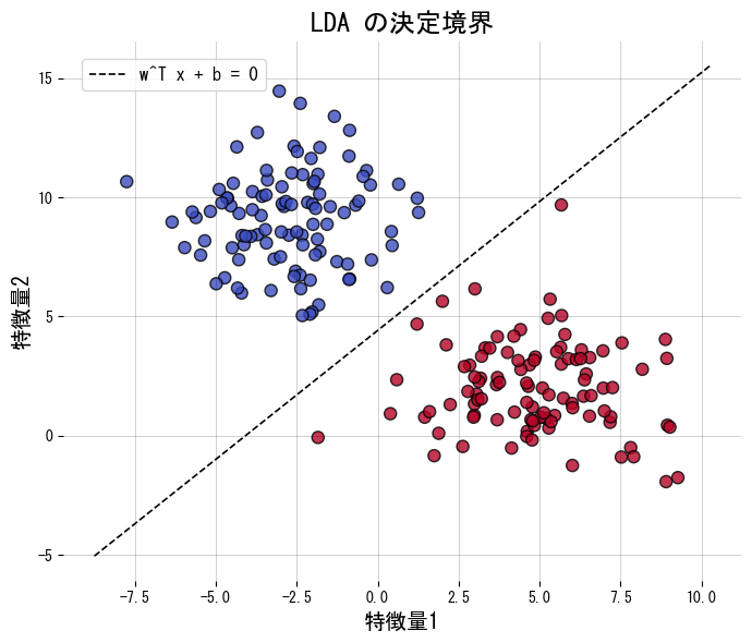
- เส้นแบ่งมีรูป \(\mathbf{w}^\top \mathbf{x} + b = 0\) ซึ่งตีความเป็นเส้นตรงหรือระนาบในมิติสูง
- หากสมมติว่าทุกคลาสเป็นแกาสเซียนที่มีเมทริกซ์โคเวเรียนซ์เท่ากันจะได้ตัวจำแนกที่เกือบเหมาะเชิงเบย์
LinearDiscriminantAnalysisใน scikit-learn ช่วยให้ฝึก วาดเส้นแบ่ง และดูฟีเจอร์หลังการฉายได้สะดวก
ภาพรวมเชิงสัญชาติญาณ #
LDA ต้องการ “กด” ตัวอย่างในคลาสเดียวกันให้เข้าใกล้ และ “ดึง” คลาสต่างกันให้ออกห่าง เมื่อฉายข้อมูลตามเวกเตอร์นั้น คลาสจะแยกจากกันได้ดีขึ้น และยังลดมิติเพื่อส่งต่อให้ตัวจำแนกอื่นได้ด้วย
สูตรสำคัญ #
ในกรณีสองคลาส เวกเตอร์ฉาย \(\mathbf{w}\) หาได้จากการเพิ่ม
$$ J(\mathbf{w}) = \frac{\mathbf{w}^\top \mathbf{S}_B \mathbf{w}}{\mathbf{w}^\top \mathbf{S}_W \mathbf{w}}, $$
โดย \(\mathbf{S}_B\) คือเมทริกซ์ความแปรปรวนระหว่างคลาส และ \(\mathbf{S}_W\) คือภายในคลาส หากมีหลายคลาสจะได้มากสุด \(K-1\) เวกเตอร์ฉาย (เมื่อมี \(K\) คลาส) ซึ่งใช้ลดมิติได้
ทดลองด้วย Python #
โค้ดต่อไปนี้ฝึก LDA กับข้อมูลสองคลาสและวาดทั้งเส้นแบ่งและผลหลังฉาย
from __future__ import annotations
import japanize_matplotlib
import matplotlib.pyplot as plt
import numpy as np
from sklearn.datasets import make_blobs
from sklearn.discriminant_analysis import LinearDiscriminantAnalysis
from sklearn.metrics import accuracy_score
def run_lda_demo(
n_samples: int = 200,
random_state: int = 42,
title_boundary: str = "เส้นแบ่งของ LDA",
title_projection: str = "การฉายด้วย LDA",
xlabel: str = "คุณลักษณะที่ 1",
ylabel: str = "คุณลักษณะที่ 2",
hist_xlabel: str = "ค่าหลังฉาย",
class0_label: str = "คลาส 0",
class1_label: str = "คลาส 1",
) -> dict[str, float]:
"""Train LDA on synthetic blobs and plot boundary plus projection."""
japanize_matplotlib.japanize()
X, y = make_blobs(
n_samples=n_samples,
centers=2,
n_features=2,
cluster_std=2.0,
random_state=random_state,
)
clf = LinearDiscriminantAnalysis(store_covariance=True)
clf.fit(X, y)
accuracy = float(accuracy_score(y, clf.predict(X)))
w = clf.coef_[0]
b = float(clf.intercept_[0])
xs = np.linspace(X[:, 0].min() - 1, X[:, 0].max() + 1, 300)
ys_boundary = -(w[0] / w[1]) * xs - b / w[1]
fig, ax = plt.subplots(figsize=(7, 6))
ax.set_title(title_boundary)
ax.scatter(X[:, 0], X[:, 1], c=y, cmap="coolwarm", edgecolor="k", alpha=0.8)
ax.plot(xs, ys_boundary, "k--", lw=1.2, label="w^T x + b = 0")
ax.set_xlabel(xlabel)
ax.set_ylabel(ylabel)
ax.legend(loc="best")
ax.grid(alpha=0.25)
fig.tight_layout()
plt.show()
X_proj = clf.transform(X)[:, 0]
fig, ax = plt.subplots(figsize=(8, 4))
ax.set_title(title_projection)
ax.hist(X_proj[y == 0], bins=20, alpha=0.7, label=class0_label)
ax.hist(X_proj[y == 1], bins=20, alpha=0.7, label=class1_label)
ax.set_xlabel(hist_xlabel)
ax.legend(loc="best")
ax.grid(alpha=0.25)
fig.tight_layout()
plt.show()
return {"accuracy": accuracy}
metrics = run_lda_demo(
title_boundary="เส้นแบ่งของ LDA",
title_projection="การฉายด้วย LDA",
xlabel="คุณลักษณะที่ 1",
ylabel="คุณลักษณะที่ 2",
hist_xlabel="ค่าหลังฉาย",
class0_label="คลาส 0",
class1_label="คลาส 1",
)
print(f"ความแม่นยำขณะฝึก: {metrics['accuracy']:.3f}")

เอกสารอ้างอิง #
- Fisher, R. A. (1936). The Use of Multiple Measurements in Taxonomic Problems. Annals of Eugenics, 7(2), 179 E88.
- Hastie, T., Tibshirani, R., & Friedman, J. (2009). The Elements of Statistical Learning. Springer.