- ลอจิสติกรีเกรสชันนำผลรวมเชิงเส้นของอินพุตผ่านฟังก์ชันซิกมอยด์เพื่อประมาณความน่าจะเป็นที่อยู่ในคลาส 1
- เอาต์พุตจำกัดอยู่ในช่วง \([0,1]\) จึงตั้ง threshold ได้ยืดหยุ่น และสัมประสิทธิ์ตีความเป็น log-odds ได้
- ฝึกด้วยการลดทอน cross-entropy (เท่ากับเพิ่มค่าความน่าจะเป็นร่วม) และสามารถเพิ่มโทษ L1/L2 เพื่อยับยั้งการเรียนรู้เกิน
LogisticRegressionใน scikit-learn ทำให้เทรนและวาดเส้นแบ่งได้ภายในไม่กี่บรรทัด
ภาพรวมเชิงสัญชาติญาณ #
การถดถอยเชิงเส้นให้ผลเป็นตัวเลขบนแกนจริง แต่หลายครั้งเราต้องการ “ความน่าจะเป็น” ที่ข้อมูลเป็นคลาสบวก ลอจิสติกรีเกรสชันคำนวณ \(z = \mathbf{w}^\top \mathbf{x} + b\) แล้วส่งผ่าน \(\sigma(z) = 1/(1 + e^{-z})\) ให้ได้ผลลัพธ์ระหว่าง 0–1 จากนั้นกำหนด threshold เช่น 0.5 เพื่อเปลี่ยนเป็นการตัดสินใจสองคลาส
สูตรสำคัญ #
ความน่าจะเป็นของคลาส 1 เมื่ออินพุตเป็น \(\mathbf{x}\) คือ
$$ P(y=1 \mid \mathbf{x}) = \sigma(\mathbf{w}^\top \mathbf{x} + b) = \frac{1}{1 + \exp\left(-(\mathbf{w}^\top \mathbf{x} + b)\right)}. $$
ค่าสัมประสิทธิ์หาได้จากการเพิ่มค่าลอการิทึมของความน่าจะเป็นร่วม
$$ \ell(\mathbf{w}, b) = \sum_{i=1}^{n} \Bigl[ y_i \log p_i + (1 - y_i) \log (1 - p_i) \Bigr], \quad p_i = \sigma(\mathbf{w}^\top \mathbf{x}_i + b), $$
ซึ่งเท่ากับการลดทอน cross-entropy ส่วนโทษ L2 ทำให้สัมประสิทธิ์ไม่พุ่งสูง ส่วน L1 สามารถกดให้บางพจน์เป็นศูนย์
ทดลองด้วย Python #
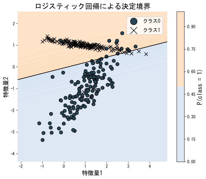
ตัวอย่างต่อไปนี้ฝึกโมเดลบนข้อมูลสองมิติที่แบ่งเส้นตรงได้ แล้ววาดเส้นแบ่งพร้อมแผนที่ความน่าจะเป็น
from __future__ import annotations
import japanize_matplotlib
import matplotlib.pyplot as plt
import numpy as np
from matplotlib.colors import ListedColormap
from sklearn.datasets import make_classification
from sklearn.linear_model import LogisticRegression
from sklearn.metrics import accuracy_score
def run_logistic_regression_demo(
n_samples: int = 300,
random_state: int = 2,
label_class0: str = "คลาส 0",
label_class1: str = "คลาส 1",
label_boundary: str = "เส้นแบ่ง",
title: str = "เส้นแบ่งจากลอจิสติกรีเกรสชัน",
) -> dict[str, float]:
"""Train logistic regression on a synthetic 2D dataset and visualise the boundary."""
japanize_matplotlib.japanize()
X, y = make_classification(
n_samples=n_samples,
n_features=2,
n_redundant=0,
n_informative=2,
random_state=random_state,
n_clusters_per_class=1,
)
clf = LogisticRegression()
clf.fit(X, y)
accuracy = float(accuracy_score(y, clf.predict(X)))
coef = clf.coef_[0]
intercept = float(clf.intercept_[0])
x1, x2 = X[:, 0], X[:, 1]
grid_x1, grid_x2 = np.meshgrid(
np.linspace(x1.min() - 1.0, x1.max() + 1.0, 200),
np.linspace(x2.min() - 1.0, x2.max() + 1.0, 200),
)
grid = np.c_[grid_x1.ravel(), grid_x2.ravel()]
probs = clf.predict_proba(grid)[:, 1].reshape(grid_x1.shape)
cmap = ListedColormap(["#aec7e8", "#ffbb78"])
fig, ax = plt.subplots(figsize=(7, 6))
contour = ax.contourf(grid_x1, grid_x2, probs, levels=20, cmap=cmap, alpha=0.4)
ax.contour(grid_x1, grid_x2, probs, levels=[0.5], colors="k", linewidths=1.5)
ax.scatter(x1[y == 0], x2[y == 0], marker="o", edgecolor="k", label=label_class0)
ax.scatter(x1[y == 1], x2[y == 1], marker="x", color="k", label=label_class1)
ax.set_xlabel("คุณลักษณะ 1")
ax.set_ylabel("คุณลักษณะ 2")
ax.set_title(title)
ax.legend(loc="best")
fig.colorbar(contour, ax=ax, label="P(class = 1)")
fig.tight_layout()
plt.show()
return {
"accuracy": accuracy,
"coef_0": float(coef[0]),
"coef_1": float(coef[1]),
"intercept": intercept,
}
metrics = run_logistic_regression_demo(
label_class0="คลาส 0",
label_class1="คลาส 1",
label_boundary="เส้นแบ่ง",
title="เส้นแบ่งจากลอจิสติกรีเกรสชัน",
)
print(f"ความแม่นยำขณะฝึก: {metrics['accuracy']:.3f}")
print(f"ค่าน้ำหนักคุณลักษณะ 1: {metrics['coef_0']:.3f}")
print(f"ค่าน้ำหนักคุณลักษณะ 2: {metrics['coef_1']:.3f}")
print(f"ไบแอส: {metrics['intercept']:.3f}")

เอกสารอ้างอิง #
- Agresti, A. (2015). Foundations of Linear and Generalized Linear Models. Wiley.
- Hastie, T., Tibshirani, R., & Friedman, J. (2009). The Elements of Statistical Learning. Springer.