まとめ
- เพอร์เซ็ปตรอนเป็นอัลกอริทึมออนไลน์เชิงคลาสสิกที่รับประกันการลู่เข้าภายในจำนวนรอบจำกัด หากข้อมูลจำแนกเชิงเส้นได้
- พยากรณ์ด้วยสัญลักษณ์ของ \(\mathbf{w}^\top \mathbf{x} + b\) และอัปเดตน้ำหนักเฉพาะเมื่อทำนายผิด
- กฎอัปเดตเรียบง่าย ทำให้จับแนวคิดการไล่ระดับและการขยับเส้นแบ่งทีละนิดผ่านอัตราเรียนรู้ได้ง่าย
- หากข้อมูลไม่เชิงเส้น ต้องขยายฟีเจอร์หรือใช้เคอร์เนลเพื่อขยายกำลังจำแนก
ภาพรวมเชิงสัญชาติญาณ #
เพอร์เซ็ปตรอนย้ายเส้นแบ่งไปทีละน้อยเมื่อพบตัวอย่างที่ทำนายผิด น้ำหนัก \(\mathbf{w}\) บอกทิศของเส้นแบ่ง ส่วนไบแอส \(b\) ขยับเส้นขึ้นหรือลง เมื่อปรับอัตราเรียนรู้ \(\eta\) เครื่องหมายของความผิดพลาดจะผลักเส้นในทิศที่ลดข้อผิดพลาด
สูตรสำคัญ #
ฟังก์ชันพยากรณ์คือ
$$ \hat{y} = \operatorname{sign}(\mathbf{w}^\top \mathbf{x} + b) $$
หากตัวอย่าง \((\mathbf{x}_i, y_i)\) ถูกจำแนกผิด ให้ปรับ
$$ \mathbf{w} \leftarrow \mathbf{w} + \eta, y_i, \mathbf{x}_i,\qquad b \leftarrow b + \eta, y_i $$
หากข้อมูลจำแนกเชิงเส้นได้ การทำซ้ำกฎนี้จะลู่เข้าภายในจำนวนก้าวจำกัด
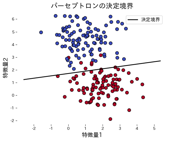
ทดลองด้วย Python #
ตัวอย่างต่อไปนี้ฝึกเพอร์เซ็ปตรอนบนข้อมูลสังเคราะห์และวาดเส้นแบ่ง
from __future__ import annotations
import japanize_matplotlib
import matplotlib.pyplot as plt
import numpy as np
from sklearn.datasets import make_blobs
from sklearn.metrics import accuracy_score
def run_perceptron_demo(
n_samples: int = 200,
lr: float = 0.1,
n_epochs: int = 20,
random_state: int = 0,
title: str = "เส้นแบ่งของเพอร์เซ็ปตรอน",
xlabel: str = "คุณลักษณะที่ 1",
ylabel: str = "คุณลักษณะที่ 2",
label_boundary: str = "เส้นแบ่ง",
) -> dict[str, object]:
"""Train a perceptron on synthetic blobs and plot the decision boundary."""
japanize_matplotlib.japanize()
X, y = make_blobs(
n_samples=n_samples,
centers=2,
cluster_std=1.0,
random_state=random_state,
)
y_signed = np.where(y == 0, -1, 1)
w = np.zeros(X.shape[1])
b = 0.0
history: list[int] = []
for _ in range(n_epochs):
errors = 0
for xi, target in zip(X, y_signed):
update = lr * target if target * (np.dot(w, xi) + b) <= 0 else 0.0
if update != 0.0:
w += update * xi
b += update
errors += 1
history.append(int(errors))
if errors == 0:
break
preds = np.where(np.dot(X, w) + b >= 0, 1, -1)
accuracy = float(accuracy_score(y_signed, preds))
xx = np.linspace(X[:, 0].min() - 1, X[:, 0].max() + 1, 200)
yy = -(w[0] * xx + b) / w[1]
fig, ax = plt.subplots(figsize=(6, 5))
ax.scatter(X[:, 0], X[:, 1], c=y, cmap="coolwarm", edgecolor="k")
ax.plot(xx, yy, color="black", linewidth=2, label=label_boundary)
ax.set_xlabel(xlabel)
ax.set_ylabel(ylabel)
ax.set_title(title)
ax.legend(loc="best")
fig.tight_layout()
plt.show()
return {"weights": w, "bias": b, "errors": history, "accuracy": accuracy}
metrics = run_perceptron_demo(
title="เส้นแบ่งของเพอร์เซ็ปตรอน",
xlabel="คุณลักษณะที่ 1",
ylabel="คุณลักษณะที่ 2",
label_boundary="เส้นแบ่ง",
)
print(f"ความแม่นยำขณะฝึก: {metrics['accuracy']:.3f}")
print("น้ำหนัก:", metrics["weights"])
print(f"ไบแอส: {metrics['bias']:.3f}")
print("จำนวนข้อผิดพลาดในแต่ละ epoch:", metrics["errors"])

เอกสารอ้างอิง #
- Rosenblatt, F. (1958). The Perceptron: A Probabilistic Model for Information Storage and Organization in the Brain. Psychological Review, 65(6), 386 E08.
- Goodfellow, I., Bengio, Y., & Courville, A. (2016). Deep Learning. MIT Press.