- SVM เรียนรู้เส้นแบ่งที่เพิ่มมาร์จินระหว่างคลาส จึงให้ความสำคัญกับการทั่วไปมากกว่าการฟิตข้อมูลฝึก
- Soft-margin SVM เพิ่มตัวแปร slack เพื่ออนุญาตให้บางจุดผิดพลาด และใช้พารามิเตอร์ \(C\) เพื่อควบคุมการลงโทษ
- Kernel trick แทนที่สเกลาร์โปรดักต์ด้วยเคอร์เนล ทำให้สร้างเส้นแบ่งไม่เชิงเส้นโดยไม่ต้องสร้างฟีเจอร์เพิ่ม
- การทำมาตรฐานและการค้นหาค่า \(C\), \(\gamma\) (หรือพารามิเตอร์เคอร์เนลอื่น) เป็นหัวใจของการได้ผลลัพธ์ที่ดี
ภาพรวมเชิงสัญชาติญาณ #
เมื่อข้อมูลแบ่งเชิงเส้นได้ SVM จะเลือกเส้นแบ่งที่ห่างจากตัวอย่างทั้งสองฝั่งมากที่สุด ตัวอย่างที่สัมผัสแถบมาร์จินเรียกว่า support vector และมีผลโดยตรงต่อเส้นแบ่ง ส่วนจุดอื่นไม่กระทบ ทำให้โมเดลนิ่งต่อ noise
สูตรสำคัญ #
กรณีแยกเชิงเส้นได้ ทำการเพิ่มประสิทธิภาพ
$$ \min_{\mathbf{w}, b} \ \frac{1}{2} \lVert \mathbf{w} \rVert_2^2 \quad \text{s.t.} \quad y_i(\mathbf{w}^\top \mathbf{x}_i + b) \ge 1. $$
สำหรับข้อมูลจริงมักต้องใช้ soft margin โดยเพิ่มตัวแปร \(\xi_i\)
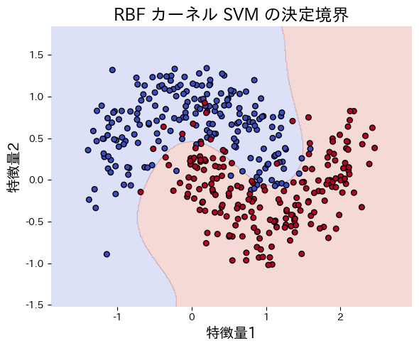
$$ \min_{\mathbf{w}, b, \boldsymbol{\xi}} \ \frac{1}{2} \lVert \mathbf{w} \rVert_2^2 + C \sum_{i=1}^{n} \xi_i \quad \text{s.t.} \quad y_i(\mathbf{w}^\top \mathbf{x}_i + b) \ge 1 - \xi_i. $$
แทนที่ \(\mathbf{x}_i^\top \mathbf{x}_j\) ด้วยเคอร์เนล \(K(\mathbf{x}_i, \mathbf{x}_j)\) เพื่อสร้างเส้นแบ่งไม่เชิงเส้นได้ เช่น RBF, Polynomial, Sigmoid
ทดลองด้วย Python #
ตัวอย่างต่อไปนี้เปรียบเทียบเส้นแบ่งของ SVM แบบเชิงเส้นและ RBF บนข้อมูล make_moons
from __future__ import annotations
import japanize_matplotlib
import matplotlib.pyplot as plt
import numpy as np
from sklearn.datasets import make_moons
from sklearn.metrics import accuracy_score
from sklearn.pipeline import make_pipeline
from sklearn.preprocessing import StandardScaler
from sklearn.svm import SVC
def run_svm_demo(
n_samples: int = 400,
noise: float = 0.25,
random_state: int = 42,
title: str = "พื้นที่การจำแนกของ SVM (RBF kernel)",
xlabel: str = "คุณลักษณะที่ 1",
ylabel: str = "คุณลักษณะที่ 2",
) -> dict[str, float]:
"""Train linear and RBF SVMs and plot the RBF decision boundary."""
japanize_matplotlib.japanize()
X, y = make_moons(n_samples=n_samples, noise=noise, random_state=random_state)
linear_clf = make_pipeline(StandardScaler(), SVC(kernel="linear", C=1.0))
linear_clf.fit(X, y)
rbf_clf = make_pipeline(StandardScaler(), SVC(kernel="rbf", C=5.0, gamma=0.5))
rbf_clf.fit(X, y)
linear_acc = float(accuracy_score(y, linear_clf.predict(X)))
rbf_acc = float(accuracy_score(y, rbf_clf.predict(X)))
grid_x, grid_y = np.meshgrid(
np.linspace(X[:, 0].min() - 0.5, X[:, 0].max() + 0.5, 400),
np.linspace(X[:, 1].min() - 0.5, X[:, 1].max() + 0.5, 400),
)
grid = np.c_[grid_x.ravel(), grid_y.ravel()]
rbf_scores = rbf_clf.predict(grid).reshape(grid_x.shape)
fig, ax = plt.subplots(figsize=(6, 5))
ax.contourf(grid_x, grid_y, rbf_scores, alpha=0.2, cmap="coolwarm")
ax.scatter(X[:, 0], X[:, 1], c=y, cmap="coolwarm", edgecolor="k", s=30)
ax.set_title(title)
ax.set_xlabel(xlabel)
ax.set_ylabel(ylabel)
fig.tight_layout()
plt.show()
return {"linear_accuracy": linear_acc, "rbf_accuracy": rbf_acc}
metrics = run_svm_demo(
title="พื้นที่การจำแนกของ SVM (RBF kernel)",
xlabel="คุณลักษณะที่ 1",
ylabel="คุณลักษณะที่ 2",
)
print(f"ความแม่นยำ SVM เชิงเส้น: {metrics['linear_accuracy']:.3f}")
print(f"ความแม่นยำ SVM แบบ RBF: {metrics['rbf_accuracy']:.3f}")

เอกสารอ้างอิง #
- Vapnik, V. (1998). Statistical Learning Theory. Wiley.
- Smola, A. J., & Schölkopf, B. (2004). A Tutorial on Support Vector Regression. Statistics and Computing, 14(3), 199 E22.