まとめ
- GMM มองข้อมูลเป็นผลรวมของการแจกแจงปกติหลายตัว จึงเป็นโมเดลกำเนิดที่บรรยายข้อมูลทั้งชุดด้วยความน่าจะเป็น
- สามารถคืน “หน้าที่รับผิดชอบ” (responsibility) หรือความน่าจะเป็นที่จุดหนึ่งมาจากคลัสเตอร์ใด ช่วยสื่อความไม่แน่นอนได้
- ปรับพารามิเตอร์ด้วยอัลกอริทึม EM และเลือกโครงสร้างโคเวเรียนซ์ (
full,tied,diag,spherical) ให้เหมาะ - ใช้เกณฑ์ BIC/AIC เพื่อเลือกจำนวนองค์ประกอบและสุ่มเริ่มต้นหลายครั้งเพื่อหลีกเลี่ยงจุดติด
ภาพรวมเชิงสัญชาติญาณ #
สมมติว่าข้อมูลมาจากแกาสเซียนหลายก้อน แต่ละก้อนมีค่าเฉลี่ยและโคเวเรียนซ์ต่างกัน k-means ให้คลาสเดียวแบบแข็ง ขณะที่ GMM ให้ความน่าจะเป็นของการเป็นสมาชิก ทำให้รู้ระดับความมั่นใจในการจัดกลุ่ม
สูตรสำคัญ #
ความน่าจะเป็นของเวกเตอร์ \(\mathbf{x}\) คือ
$$ p(\mathbf{x}) = \sum_{k=1}^{K} \pi_k , \mathcal{N}(\mathbf{x} \mid \boldsymbol{\mu}_k, \boldsymbol{\Sigma}_k), $$
โดย \(\pi_k\) เป็นค่าน้ำหนัก (รวมเป็น 1), \(\boldsymbol{\mu}_k\) ค่าเฉลี่ย และ \(\boldsymbol{\Sigma}_k\) เมทริกซ์โคเวเรียนซ์ EM algorithm ทำสองขั้นตอนสลับกัน:
- E-step: คำนวณความรับผิดชอบ $$ \gamma_{ik} = \frac{\pi_k , \mathcal{N}(\mathbf{x}_i \mid \boldsymbol{\mu}_k, \boldsymbol{\Sigma}k)} {\sum{j=1}^K \pi_j , \mathcal{N}(\mathbf{x}_i \mid \boldsymbol{\mu}_j, \boldsymbol{\Sigma}_j)}. $$
- M-step: ใช้ \(\gamma_{ik}\) ปรับ \(\pi_k, \boldsymbol{\mu}_k, \boldsymbol{\Sigma}_k\)
ทดลองด้วย Python #
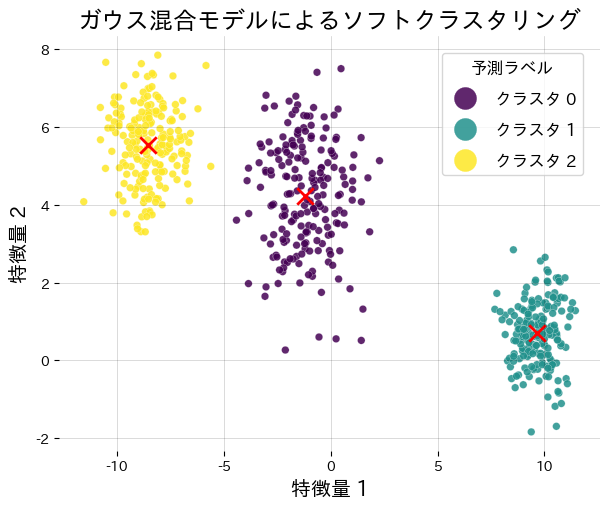
ตัวอย่างต่อไปนี้เรียนรู้ GMM 3 คลัสเตอร์และวาดศูนย์กลางพร้อมรายงานความรับผิดชอบ
from __future__ import annotations
import japanize_matplotlib
import matplotlib.pyplot as plt
import numpy as np
from numpy.typing import NDArray
from sklearn.datasets import make_blobs
from sklearn.mixture import GaussianMixture
def run_gmm_demo(
n_samples: int = 600,
n_components: int = 3,
cluster_std: list[float] | tuple[float, ...] = (1.0, 1.4, 0.8),
covariance_type: str = "full",
random_state: int = 7,
n_init: int = 8,
) -> dict[str, object]:
"""เรียนรู้ Gaussian Mixture และแสดงศูนย์กลางกับหน้าที่รับผิดชอบ."""
japanize_matplotlib.japanize()
features, labels_true = make_blobs(
n_samples=n_samples,
centers=n_components,
cluster_std=cluster_std,
random_state=random_state,
)
gmm = GaussianMixture(
n_components=n_components,
covariance_type=covariance_type,
random_state=random_state,
n_init=n_init,
)
gmm.fit(features)
hard_labels = gmm.predict(features)
responsibilities = gmm.predict_proba(features)
log_likelihood = float(gmm.score(features))
weights = gmm.weights_
fig, ax = plt.subplots(figsize=(6.2, 5.2))
scatter = ax.scatter(
features[:, 0],
features[:, 1],
c=hard_labels,
cmap="viridis",
s=30,
edgecolor="white",
linewidth=0.2,
alpha=0.85,
)
ax.scatter(
gmm.means_[:, 0],
gmm.means_[:, 1],
marker="x",
c="red",
s=140,
linewidth=2.0,
label="ศูนย์กลางคลัสเตอร์",
)
ax.set_title("Soft clustering ด้วย Gaussian Mixture")
ax.set_xlabel("คุณลักษณะที่ 1")
ax.set_ylabel("คุณลักษณะที่ 2")
ax.grid(alpha=0.2)
handles, _ = scatter.legend_elements()
labels = [f"คลัสเตอร์ {idx}" for idx in range(n_components)]
ax.legend(handles, labels, title="ป้ายที่พยากรณ์", loc="upper right")
fig.tight_layout()
plt.show()
return {
"log_likelihood": log_likelihood,
"weights": weights.tolist(),
"responsibilities_shape": responsibilities.shape,
}
metrics = run_gmm_demo()
print(f"ค่า log-likelihood: {metrics['log_likelihood']:.3f}")
print("ค่าน้ำหนักของส่วนผสม:", metrics["weights"])
print("รูปทรงของเมทริกซ์หน้าที่รับผิดชอบ:", metrics["responsibilities_shape"])

เอกสารอ้างอิง #
- Bishop, C. M. (2006). Pattern Recognition and Machine Learning. Springer.
- Dempster, A. P., Laird, N. M., & Rubin, D. B. (1977). Maximum Likelihood from Incomplete Data via the EM Algorithm. Journal of the Royal Statistical Society, Series B.
- scikit-learn developers. (2024). Gaussian Mixture Models. https://scikit-learn.org/stable/modules/mixture.html