まとめ
- WLS ให้ค่าน้ำหนักกับแต่ละการสังเกตตามความเชื่อถือ จึงประมาณเส้นถดถอยได้ดีแม้ noise ไม่เท่ากัน
- การคูณน้ำหนักกับกำลังสองของส่วนคลาดเคลื่อนทำให้จุดที่มีความแปรปรวนต่ำส่งผลมากกว่า และไม่ถูกลากด้วยจุดที่ noisy
LinearRegressionของscikit-learnรองรับ WLS เพียงระบุsample_weight- น้ำหนักอาจมาจากความรู้โดเมน การคาดประมาณความแปรปรวน หรือจากการวิเคราะห์ residual
ภาพรวมเชิงสัญชาติญาณ #
วิธีกำลังสองน้อยที่สุดปฏิบัติต่อทุกจุดเหมือนกัน แต่ในข้อมูลจริงแหล่งที่มาบางช่วงอาจแม่นยำกว่าช่วงอื่น WLS จึง “ให้เสียงที่ดังขึ้น” กับจุดที่น่าเชื่อถือกว่า ในขณะที่จุดที่ noisy ถูกกดน้ำหนักลง
สูตรสำคัญ #
ให้ค่าน้ำหนัก \(w_i > 0\) กับแต่ละการสังเกตแล้วทำให้
$$ L(\boldsymbol\beta, b) = \sum_{i=1}^{n} w_i \left(y_i - (\boldsymbol\beta^\top \mathbf{x}_i + b)\right)^2 $$
ต่ำสุด หากทราบความแปรปรวน \(\sigma_i^2\) ของแต่ละจุดล่วงหน้า ค่าน้ำหนักที่เหมาะคือ \(w_i \propto 1/\sigma_i^2\)
ทดลองด้วย Python #
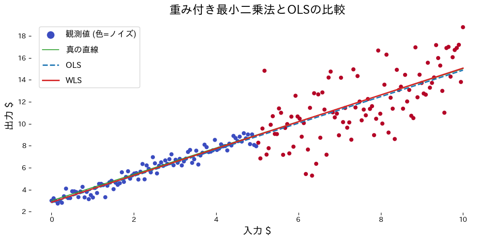
ตัวอย่างต่อไปนี้สร้างข้อมูลที่ครึ่งหนึ่งมี noise ต่ำ อีกครึ่ง noise สูง แล้วเปรียบเทียบ OLS กับ WLS
from __future__ import annotations
import japanize_matplotlib
import matplotlib.pyplot as plt
import numpy as np
from sklearn.linear_model import LinearRegression
def run_weighted_vs_ols(
n_samples: int = 200,
threshold: float = 5.0,
low_noise: float = 0.5,
high_noise: float = 2.5,
xlabel: str = "input $x$",
ylabel: str = "output $y$",
label_scatter: str = "observations (color=noise)",
label_truth: str = "true line",
label_ols: str = "OLS",
label_wls: str = "WLS",
title: str | None = None,
) -> dict[str, float]:
"""Compare OLS and weighted least squares on heteroscedastic data."""
japanize_matplotlib.japanize()
rng = np.random.default_rng(7)
X_vals: np.ndarray = np.linspace(0.0, 10.0, n_samples, dtype=float)
true_y: np.ndarray = 1.2 * X_vals + 3.0
noise_scale = np.where(X_vals < threshold, low_noise, high_noise)
y_noisy = true_y + rng.normal(scale=noise_scale)
weights = 1.0 / (noise_scale**2)
X = X_vals[:, np.newaxis]
ols = LinearRegression()
ols.fit(X, y_noisy)
wls = LinearRegression()
wls.fit(X, y_noisy, sample_weight=weights)
grid = np.linspace(0.0, 10.0, 200, dtype=float)[:, np.newaxis]
ols_pred = ols.predict(grid)
wls_pred = wls.predict(grid)
fig, ax = plt.subplots(figsize=(10, 5))
scatter = ax.scatter(
X,
y_noisy,
c=noise_scale,
cmap="coolwarm",
s=25,
label=label_scatter,
)
ax.plot(grid, 1.2 * grid.ravel() + 3.0, color="#2ca02c", label=label_truth)
ax.plot(grid, ols_pred, color="#1f77b4", linestyle="--", linewidth=2, label=label_ols)
ax.plot(grid, wls_pred, color="#d62728", linewidth=2, label=label_wls)
ax.set_xlabel(xlabel)
ax.set_ylabel(ylabel)
if title:
ax.set_title(title)
ax.legend()
fig.tight_layout()
plt.show()
return {
"ols_slope": float(ols.coef_[0]),
"ols_intercept": float(ols.intercept_),
"wls_slope": float(wls.coef_[0]),
"wls_intercept": float(wls.intercept_),
}
metrics = run_weighted_vs_ols(
xlabel="อินพุต $x$",
ylabel="เอาต์พุต $y$",
label_scatter="จุดสังเกต (สี=ระดับ noise)",
label_truth="เส้นจริง",
label_ols="OLS",
label_wls="WLS",
title="เปรียบเทียบ OLS กับ Weighted Least Squares",
)
print(f"OLS: slope = {metrics['ols_slope']:.3f}, intercept = {metrics['ols_intercept']:.3f}")
print(f"WLS: slope = {metrics['wls_slope']:.3f}, intercept = {metrics['wls_intercept']:.3f}")

วิเคราะห์ผลลัพธ์ #
- เมื่อเติมน้ำหนักตามความแปรปรวน จุดที่ noise ต่ำมีอิทธิพลมากขึ้น เส้น WLS จึงเข้าใกล้เส้นจริงกว่า OLS
- OLS ถูกลากไปตามส่วนที่ noise สูง ผลคือความชันต่ำเกินจริง
- การออกแบบน้ำหนักอย่างเหมาะสมเป็นหัวใจของ WLS อาจใช้สูตรจากทฤษฎีหรือประเมินจาก residual ก็ได้
เอกสารอ้างอิง #
- Carroll, R. J., & Ruppert, D. (1988). Transformation and Weighting in Regression. Chapman & Hall.
- Seber, G. A. F., & Lee, A. J. (2012). Linear Regression Analysis (2nd ed.). Wiley.