2.3.1
Decision Tree (Classifier)
- Decision tree classifier แบ่งพื้นที่ฟีเจอร์ด้วยคำถามแบบ if-then จนถึงใบไม้ที่มีคลาสเด่นชัด
- ใช้เกณฑ์อย่าง Gini หรือ entropy เพื่อวัดคุณภาพของการแบ่ง
- ปรับความลึกและขนาดใบเพื่อลด overfitting แต่ยังคงความสามารถในการอธิบายผล
- การวาดขอบเขตการตัดสินใจและโครงสร้างต้นไม้ช่วยสื่อสารกับผู้เกี่ยวข้องได้ง่าย
สัญชาตญาณ #
การเข้าใจวิธีนี้ควรดูสมมติฐานของโมเดล ลักษณะข้อมูล และผลของการตั้งค่าพารามิเตอร์ต่อการทั่วไปของโมเดล
คำอธิบายโดยละเอียด #
1. ภาพรวม #
ต้นไม้ตัดสินใจเป็นโมเดลที่แบ่งพื้นที่อินพุตแบบวนซ้ำ โดยโหนดแต่ละจุดถามคำถามเช่น “(x_j \le s) หรือไม่?” สำหรับงานจำแนก เราต้องการให้ใบไม้มีความบริสุทธิ์สูง เพื่อให้ผลทำนายมีความชัดเจน โมเดลจึงทำหน้าที่เหมือนชุดกฎที่ตรวจสอบได้ง่าย
2. ตัวชี้วัดความไม่บริสุทธิ์ #
ให้ (t) เป็นโหนด และ (p_k) เป็นสัดส่วนของคลาส (k) ภายในโหนดนั้น
$$ \mathrm{Gini}(t) = 1 - \sum_k p_k^2, $$$$ H(t) = - \sum_k p_k \log p_k. $$ถ้าแบ่งโหนด (t) ด้วยฟีเจอร์ (x_j) และค่า (s) จะได้การลดความไม่บริสุทธิ์เป็น
$$ \Delta I = I(t) - \frac{n_L}{n_t} I(t_L) - \frac{n_R}{n_t} I(t_R), $$โดย (I(\cdot)) คือ Gini หรือ entropy, (t_L), (t_R) คือโหนดย่อย และ (n_t) คือจำนวนตัวอย่าง ระบบจะเลือก split ที่ทำให้ (\Delta I) สูงสุด
3. ตัวอย่าง Python #
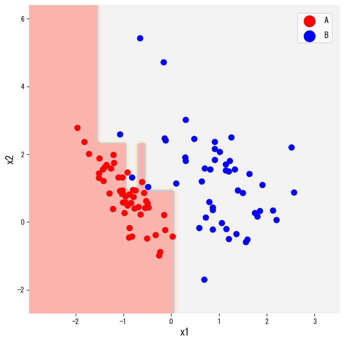
โค้ดด้านล่างสร้างข้อมูลสองคลาสด้วย make_classification แล้วฝึก DecisionTreeClassifier
จากนั้นวาดขอบเขตการตัดสินใจ โดยเปลี่ยน criterion เป็น "entropy" จะสลับไปใช้ entropy
| |
ต้นไม้ยังสามารถวาดเป็นแผนภาพด้วย plot_tree เพื่อใช้ในรายงานได้
| |

4. อ้างอิง #
- Breiman, L., Friedman, J. H., Olshen, R. A., & Stone, C. J. (1984). Classification and Regression Trees. Wadsworth.
- scikit-learn developers. (2024). Decision Trees. https://scikit-learn.org/stable/modules/tree.html