- ต้นไม้สำหรับถดถอยแบ่งพื้นที่ฟีเจอร์เป็นช่วง ๆ แล้วทำนายด้วยค่าคงที่ในแต่ละใบ
- การแบ่งเลือกจากการลด MSE ระหว่างโหนดซ้ายและขวา
- พารามิเตอร์อย่าง
max_depth,min_samples_leaf, และccp_alphaช่วยบาลานซ์ความแม่นยำกับการอธิบาย - การวาดกราฟช่วยอธิบายว่าบริเวณใดได้ค่าทำนายเหมือนกัน
1. ภาพรวม #
เหมือนกับตัวจำแนก ต้นไม้ถดถอยถามคำถามง่าย ๆ จากฟีเจอร์ แต่เป้าหมายเป็นค่าต่อเนื่อง ใบไม้จะทำนายค่าคงที่ (ค่าเฉลี่ยของตัวอย่างที่ตกมาในใบนั้น) ยิ่งลึกยิ่งจับรายละเอียดได้มาก แต่เสี่ยง overfitting มากขึ้น
2. เกณฑ์การแบ่ง (ลดความแปรปรวน) #
ให้โหนด (t) มี (n_t) ตัวอย่าง และค่าเฉลี่ยเป้าหมาย (\bar{y}_t)
$$ \mathrm{MSE}(t) = \frac{1}{n_t} \sum_{i \in t} (y_i - \bar{y}_t)^2. $$
เมื่อแบ่งด้วย (x_j) ที่ค่า (s) จะได้โหนดย่อย (t_L), (t_R) และคำนวณ
$$ \Delta = \mathrm{MSE}(t) - \frac{n_L}{n_t} \mathrm{MSE}(t_L) - \frac{n_R}{n_t} \mathrm{MSE}(t_R). $$
เลือก split ที่ทำให้ (\Delta) มากที่สุด และหากไม่เพิ่มขึ้น โหนดจะกลายเป็นใบไม้
3. ตัวอย่าง Python #
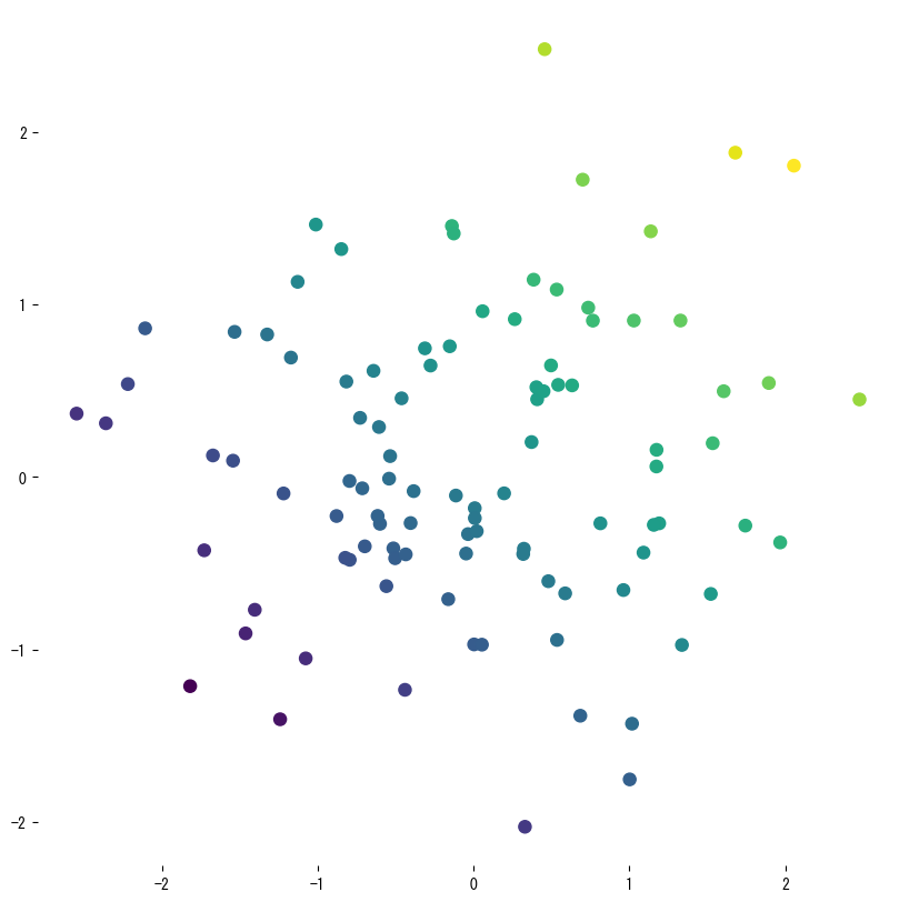
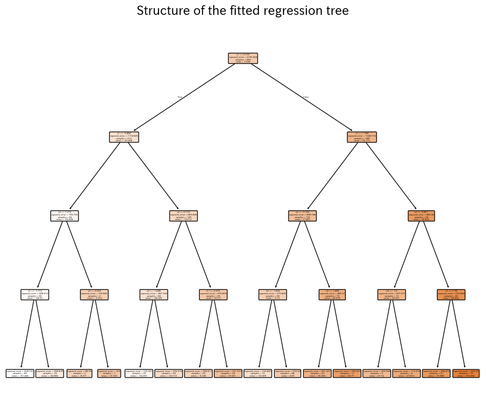
ตัวอย่างแรกสร้างข้อมูลจากเส้น sine แล้วฝึกต้นไม้ตื้น ๆ เพื่อให้เห็นการทำนายแบบขั้นบันได ตัวอย่างที่สองฝึกต้นไม้ด้วยฟีเจอร์ 2 ตัว แล้ววัด (R^2), RMSE, MAE พร้อมวาดพื้นผิวทำนาย
import numpy as np
import matplotlib.pyplot as plt
from sklearn.tree import DecisionTreeRegressor, plot_tree
from sklearn.datasets import make_regression
from sklearn.metrics import r2_score, mean_squared_error, mean_absolute_error
rng = np.random.default_rng(42)
X1 = np.sort(5 * rng.random((120, 1)), axis=0)
y1_true = np.sin(X1).ravel()
y1 = y1_true + rng.normal(scale=0.2, size=X1.shape[0])
reg1 = DecisionTreeRegressor(max_depth=3, random_state=0).fit(X1, y1)
y1_pred = reg1.predict(X1)
plt.figure(figsize=(8, 4))
plt.scatter(X1, y1, s=15, c="gray", label="observations")
plt.plot(X1, y1_true, lw=2, label="true signal")
plt.step(X1.ravel(), y1_pred, where="mid", lw=2, label="tree prediction")
plt.xlabel("x")
plt.ylabel("y")
plt.title("Piecewise-constant fit by a regression tree")
plt.legend()
plt.grid(alpha=0.3)
plt.show()

X, y = make_regression(n_samples=400, n_features=2, noise=15.0, random_state=777)
reg = DecisionTreeRegressor(max_depth=4, random_state=0).fit(X, y)
r2 = r2_score(y, reg.predict(X))
rmse = mean_squared_error(y, reg.predict(X), squared=False)
mae = mean_absolute_error(y, reg.predict(X))
print(f"R2={r2:.3f} RMSE={rmse:.2f} MAE={mae:.2f}")
x_min, x_max = X[:, 0].min()-1, X[:, 0].max()+1
y_min, y_max = X[:, 1].min()-1, X[:, 1].max()+1
xx, yy = np.meshgrid(
np.linspace(x_min, x_max, 150),
np.linspace(y_min, y_max, 150),
)
zz = reg.predict(np.c_[xx.ravel(), yy.ravel()]).reshape(xx.shape)
plt.figure(figsize=(7, 6))
cs = plt.contourf(xx, yy, zz, levels=15, cmap="viridis", alpha=0.8)
plt.colorbar(cs, label="prediction")
plt.scatter(X[:, 0], X[:, 1], c=y, cmap="viridis", s=20, edgecolor="k", alpha=0.7)
plt.xlabel("x1")
plt.ylabel("x2")
plt.title("Prediction surface of the regression tree")
plt.show()

plt.figure(figsize=(12, 10))
plot_tree(
reg,
filled=True,
feature_names=["x1", "x2"],
rounded=True,
)
plt.title("Structure of the fitted regression tree")
plt.show()

4. อ้างอิง #
- Breiman, L., Friedman, J. H., Olshen, R. A., & Stone, C. J. (1984). Classification and Regression Trees. Wadsworth.
- scikit-learn developers. (2024). Decision Trees. https://scikit-learn.org/stable/modules/tree.html