ใส่คำอธิบายลงบนสแคตเตอร์ตามหมวดหมู่

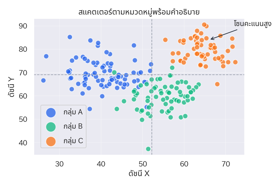
import numpy as np
import matplotlib.pyplot as plt

rng = np.random.default_rng(0)
cluster = np.concatenate([np.full(80, "A"), np.full(70, "B"), np.full(60, "C")])
x = np.concatenate([rng.normal(40, 6, 80), rng.normal(55, 5, 70), rng.normal(65, 4, 60)])
y = np.concatenate([rng.normal(70, 5, 80), rng.normal(60, 6, 70), rng.normal(80, 5, 60)])
palette = {"A": "#2563eb", "B": "#10b981", "C": "#f97316"}

fig, ax = plt.subplots(figsize=(6, 4))
for cat in np.unique(cluster):
    mask = cluster == cat
    ax.scatter(x[mask], y[mask], label=f"กลุ่ม {cat}", color=palette[cat], alpha=0.75, edgecolors="white", s=60)

ax.axvline(np.mean(x), color="#9ca3af", linestyle="--", linewidth=1)
ax.axhline(np.mean(y), color="#9ca3af", linestyle="--", linewidth=1)

ax.annotate(
    "โซนคะแนนสูง",
    xy=(66, 84),
    xytext=(72, 90),
    arrowprops=dict(arrowstyle="->", color="#1f2937"),
    fontsize=11,
)

ax.set_xlabel("ดัชนี X")
ax.set_ylabel("ดัชนี Y")
ax.set_title("สแคตเตอร์ตามหมวดหมู่พร้อมคำอธิบาย")
ax.legend()
ax.grid(alpha=0.3)

fig.tight_layout()

plt.show()