まとめ 動的時間伸縮(Dynamic Time Warping, DTW)は時間軸のずれを許容しながら 2 つの時系列の距離を最小化する整列アルゴリズム。 距離行列と累積コスト行列を動的計画法で計算し、最小コスト経路(ワーピングパス)を復元して類似度を求める。 Python で素朴な DTW を実装し、fastdtw の近似と比較しながら波形の形状が似ているかを確認する。
動的時間伸縮とは
# Dynamic Time Warping(DTW)は、時系列同士の類似度を測る際に時間軸の伸縮を許容して整列させる手法です。同じ形状でも開始タイミングや速度が異なるとユークリッド距離では大きな差になりますが、DTW なら時間軸を引き伸ばして「もっとも形が似る整列」を見つけられます。
代表的な用途:
音声・手書き文字認識:発話速度や書き順の違いを吸収してパターンマッチング。 センサーデータの異常検知:製造ラインなど周期が揺れる信号を比較。 レコメンド:ユーザー行動の経時パターンを比較し、似た行動を持つユーザーや商品の距離を測定。 アルゴリズムの流れ
# 2 本の時系列 \(X = (x_1, \dots, x_n)\)、\(Y = (y_1, \dots, y_m)\) に対して、DTW 距離は以下の手順で求めます。
距離行列の作成 累積コストの計算 ワーピングパスの復元 距離の取得 計算量は \(O(nm)\)。系列が長い場合は Sakoe–Chiba バンドなどの制約を組み合わせたり、fastdtw のような近似法を用いたりします。
NumPy で DTW を実装する
# 1
2
3
4
5
6
7
8
9
10
11
12
13
14
15
16
17
18
19
20
21
22
23
24
25
26
27
28
29
30
31
32
33
import numpy as np
def dtw_distance (
x : np . ndarray ,
y : np . ndarray ,
window : int | None = None ,
) -> tuple [ float , list [ tuple [ int , int ]]]:
n , m = len ( x ), len ( y )
window = max ( window or max ( n , m ), abs ( n - m ))
cost = np . full (( n + 1 , m + 1 ), np . inf )
cost [ 0 , 0 ] = 0.0
for i in range ( 1 , n + 1 ):
for j in range ( max ( 1 , i - window ), min ( m + 1 , i + window + 1 )):
dist = abs ( x [ i - 1 ] - y [ j - 1 ])
cost [ i , j ] = dist + min ( cost [ i - 1 , j ], cost [ i , j - 1 ], cost [ i - 1 , j - 1 ])
i , j = n , m
path : list [ tuple [ int , int ]] = []
while i > 0 and j > 0 :
path . append (( i - 1 , j - 1 ))
idx = np . argmin (( cost [ i - 1 , j ], cost [ i , j - 1 ], cost [ i - 1 , j - 1 ]))
if idx == 0 :
i -= 1
elif idx == 1 :
j -= 1
else :
i -= 1
j -= 1
path . reverse ()
return cost [ n , m ], path
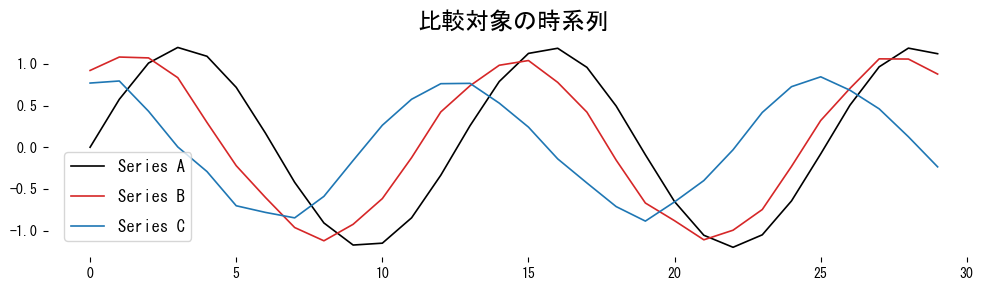
例: 3 本の波形を比較する
# 1
2
python --version # 例: Python 3.13.0
pip install matplotlib fastdtw
1
2
3
4
5
6
7
8
9
10
11
12
13
14
15
16
17
18
import matplotlib.pyplot as plt
from fastdtw import fastdtw
np . random . seed ( 42 )
time = np . arange ( 0 , 30 )
series_a = 1.2 * np . sin ( time / 2.0 )
series_b = 1.1 * np . sin (( time + 2 ) / 2.1 ) + 0.05 * np . random . randn ( len ( time ))
series_c = 0.8 * np . cos ( time / 2.0 ) + 0.05 * np . random . randn ( len ( time ))
plt . figure ( figsize = ( 10 , 3 ))
plt . plot ( time , series_a , label = "Series A" , color = "black" )
plt . plot ( time , series_b , label = "Series B" , color = "tab:red" )
plt . plot ( time , series_c , label = "Series C" , color = "tab:blue" )
plt . title ( "比較対象の時系列" )
plt . legend ()
plt . tight_layout ()
plt . show ()
 1
 2
 3
 4
 5
 6
 7
 8
 9
10
# 素朴な DTW
dist_ab , path_ab = dtw_distance ( series_a , series_b )
dist_ac , path_ac = dtw_distance ( series_a , series_c )
# 近似 DTW(fastdtw)
fast_dist_ab , _ = fastdtw ( series_a , series_b )
fast_dist_ac , _ = fastdtw ( series_a , series_c )
print ( f "DTW(A, B) = { dist_ab : .3f } / fastdtw = { fast_dist_ab : .3f } " )
print ( f "DTW(A, C) = { dist_ac : .3f } / fastdtw = { fast_dist_ac : .3f } " )
1
2
DTW(A, B)  = 5.020  / fastdtw = 5.020
DTW(A, C)  = 10.194 / fastdtw = 10.194
Series B は振幅と位相がわずかに違うだけで形状は似ているため、DTW 距離が小さくなります。Series C は波形が異なるため距離が大きくなり、fastdtw の近似もほぼ同じ値を返します。
ワーピングパスを可視化する
# 1
2
3
4
5
6
7
8
9
10
11
12
13
14
15
16
17
18
19
20
21
22
23
24
25
26
27
28
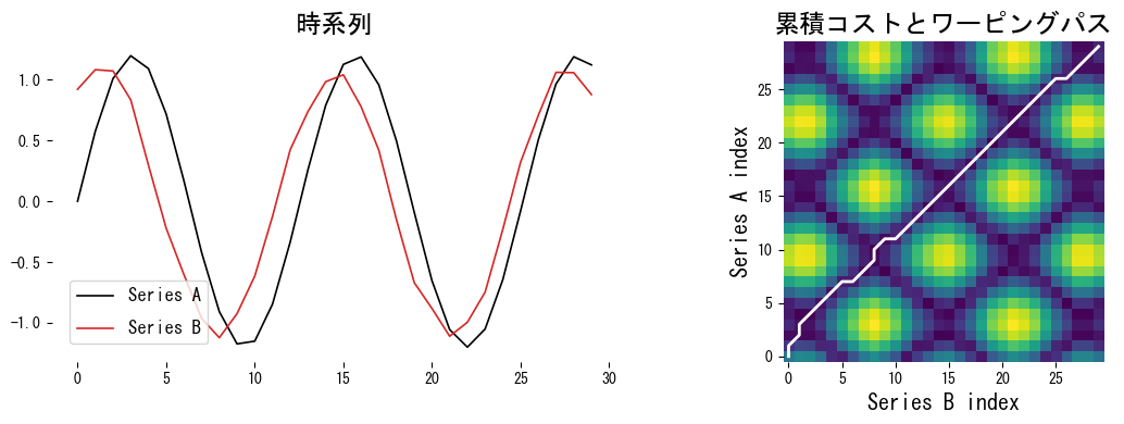
def plot_warping ( a : np . ndarray , b : np . ndarray , path : list [ tuple [ int , int ]]) -> None :
fig , axes = plt . subplots (
1 ,
2 ,
figsize = ( 12 , 4 ),
gridspec_kw = { "width_ratios" : [ 1 , 1.2 ]},
)
axes [ 0 ] . plot ( a , label = "Series A" , color = "black" )
axes [ 0 ] . plot ( b , label = "Series B" , color = "tab:red" )
axes [ 0 ] . set_title ( "時系列" )
axes [ 0 ] . legend ()
axes [ 1 ] . imshow (
np . abs ( np . subtract . outer ( a , b )),
origin = "lower" ,
interpolation = "nearest" ,
cmap = "viridis" ,
)
path_arr = np . array ( path )
axes [ 1 ] . plot ( path_arr [:, 1 ], path_arr [:, 0 ], color = "white" , linewidth = 2 )
axes [ 1 ] . set_title ( "累積コストとワーピングパス" )
axes [ 1 ] . set_xlabel ( "Series B index" )
axes [ 1 ] . set_ylabel ( "Series A index" )
plt . tight_layout ()
plt . show ()
plot_warping ( series_a , series_b , path_ab )
白線で示したワーピングパスは、Series A の遅れた山と Series B の進んだ山を対応づけており、時間軸がずれていても形状が似ていれば距離が小さくなることが分かります。
まとめ
# DTW は時間軸の伸縮を許容して時系列を整列させることで、形状の類似度を測る。 動的計画法で累積コストとワーピングパスを求めるのが基本。制約や近似法で高速化も可能。 Python では NumPy で素朴な実装が可能で、fastdtw などを組み合わせれば実務でも扱いやすい。