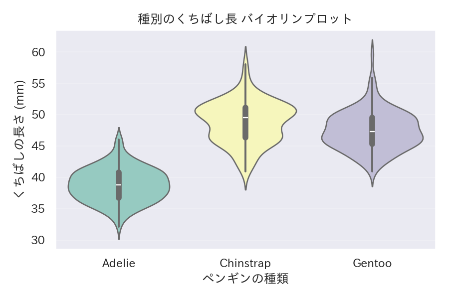
バイオリンプロット

バイオリンプロットは箱ひげ図に KDE を重ねたようなチャートで、分布の形状と外れ値を同時に把握できます。

 1
 2
 3
 4
 5
 6
 7
 8
 9
10
11
12
13
14
15

import seaborn as sns
import matplotlib.pyplot as plt

penguins = sns.load_dataset("penguins").dropna(subset=["bill_length_mm", "species"])

fig, ax = plt.subplots(figsize=(6, 4))
sns.violinplot(data=penguins, x="species", y="bill_length_mm", palette="Set3", ax=ax)
ax.set_xlabel("ペンギンの種類")
ax.set_ylabel("くちばしの長さ (mm)")
ax.set_title("種別のくちばし長 バイオリンプロット")
ax.grid(axis="y", alpha=0.2)

fig.tight_layout()

plt.show()

読み方のポイント #

• バイオリンの幅が広い部分はデータが密集している。箱ひげ図より滑らかに分布を表現できる。
• 中央の白い点線は中央値と四分位範囲を示す。箱ひげ図と同時に表示すると解釈しやすい。
• カテゴリが多い場合は横向きにするか、色数を絞って視認性を保つ。

いつ使うか #

• 適している場面: 分布の形状（多峰性や裾の重さ）をカテゴリ間で比較したいとき。箱ひげ図より情報量が多い表現です。
• 不向きな場面: カテゴリ数が多い（10以上）と図が窮屈になり、かえって読みにくくなります。
• 代替手段: リッジラインプロットならカテゴリ数が多くても縦に並べて見やすく比較できます。

よくある失敗パターン #

• KDE の裾がデータ範囲外に広がる: KDE のスムージングにより、0 以上しかとらないデータでも負の領域に密度が描かれることがあります。cut パラメータで制限してください。
• サンプルサイズの違いを無視: サンプル数が大きく異なるグループを同じ幅で描くと、少数データの分布が過剰に滑らかに見えます。サンプルサイズを注記しましょう。