まとめ- matplotlibの凡例の位置・表示対象・見た目を自在にカスタマイズする。
bbox_to_anchor や fig.legend で凡例をプロット外に配置し重なりを防ぐ。- 複数系列やサブプロットを含む図を見やすく仕上げたいときに使う。
plt.legend() を少し工夫するだけで、図の読みやすさが大きく変わります。ここでは「凡例が図と重なる」「情報が多くて読めない」といった悩みを解消する小技を、コードと出力例つきで紹介します。すべて plt.tight_layout() を入れてレイアウトを整え、凡例がプロットと重ならないよう bbox_to_anchor などで調整しています。
サンプルデータ
#
 1
 2
 3
 4
 5
 6
 7
 8
 9
10
| import numpy as np
import matplotlib.pyplot as plt
x = np.linspace(0, 2*np.pi, 200)
series = {
"sin": np.sin(x),
"cos": np.cos(x),
"sin+cos": np.sin(x) + np.cos(x),
"sin-cos": np.sin(x) - np.cos(x),
}
|
1. 位置を自由に調整 (loc + bbox_to_anchor)
#
 1
 2
 3
 4
 5
 6
 7
 8
 9
10
11
12
13
| fig, ax = plt.subplots(figsize=(8, 4))
for label, y in series.items():
ax.plot(x, y, label=label)
ax.legend(
loc="upper center",
bbox_to_anchor=(0.5, 1.18),
ncol=2,
frameon=False,
)
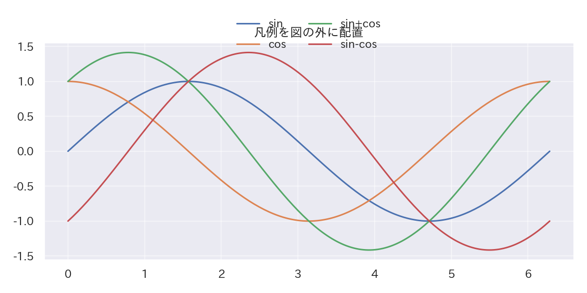
ax.set_title("凡例を図の外に配置")
plt.tight_layout()
plt.show()
|
loc で基準位置を、bbox_to_anchor でオフセットを指定すると図の外へ逃がせます。- 項目数が多いときは
ncol で列数を増やして幅を抑えると視認性が向上します。

2. 表示対象と順番を制御
#
 1
 2
 3
 4
 5
 6
 7
 8
 9
10
11
12
13
| fig, ax = plt.subplots(figsize=(8, 4))
handle_map = {}
for label, y in series.items():
handle_map[label] = ax.plot(x, y, label=label)[0]
order = ["sin+cos", "sin", "cos"]
handles = [handle_map[k] for k in order]
labels = ["合成波", "サイン", "コサイン"]
ax.legend(handles, labels, title="注目シリーズ", loc="lower right")
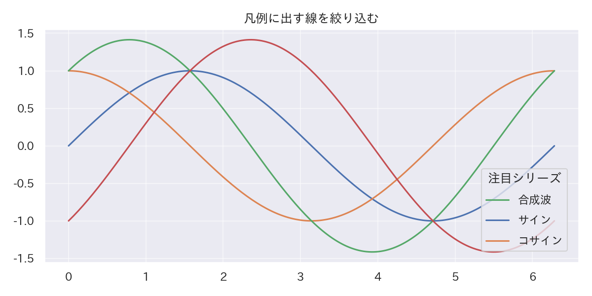
ax.set_title("凡例に出す線を絞り込む")
plt.tight_layout()
plt.show()
|
- Line2D を保持しておけば、凡例の表示対象や順序を自在にコントロールできます。
- ラベルを日本語に差し替えたい場合にもこの方法が便利です。
3. 背景・枠線を整える
#
 1
 2
 3
 4
 5
 6
 7
 8
 9
10
11
12
13
14
15
16
17
18
| fig, ax = plt.subplots(figsize=(8, 4))
for label, y in series.items():
ax.plot(x, y, linewidth=2, label=label)
legend = ax.legend(
loc="upper left",
bbox_to_anchor=(0.02, 0.98),
frameon=True,
facecolor="white",
edgecolor="#cbd5e1",
)
legend.get_frame().set_alpha(0.9)
legend.get_frame().set_linewidth(0.8)
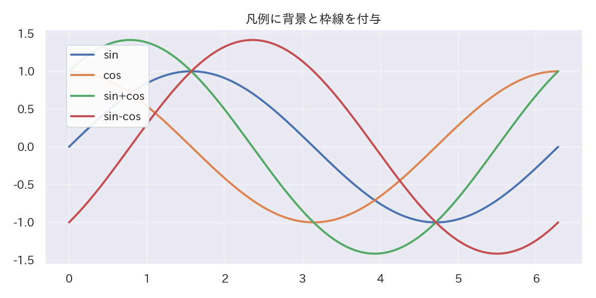
ax.set_title("凡例に背景と枠線を付与")
ax.grid(alpha=.3)
plt.tight_layout()
plt.show()
|
legend.get_frame() で FancyBboxPatch を取得し、透明度・枠線を調整できます。- 背景がごちゃつく場合、凡例を白背景にして少し浮かせると読みやすくなります。
4. サブプロット共通の凡例 (fig.legend)
#
 1
 2
 3
 4
 5
 6
 7
 8
 9
10
11
12
13
14
15
| fig, axes = plt.subplots(1, 2, figsize=(10, 4), sharey=True)
for ax, factor in zip(axes, [1.0, 0.5]):
for label, y in series.items():
ax.plot(x, factor * y, label=label)
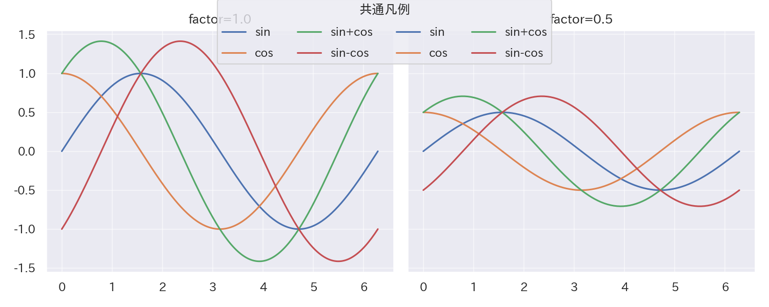
ax.set_title(f"factor={factor}")
fig.legend(
loc="upper center",
bbox_to_anchor=(0.5, 1.04),
ncol=4,
title="共通凡例",
)
fig.tight_layout()
plt.show()
|
- 複数サブプロットで同じ凡例を繰り返すと邪魔なので、
fig.legend でまとめて配置。 - ダッシュボード風に図を並べるときの定番テクニックです。
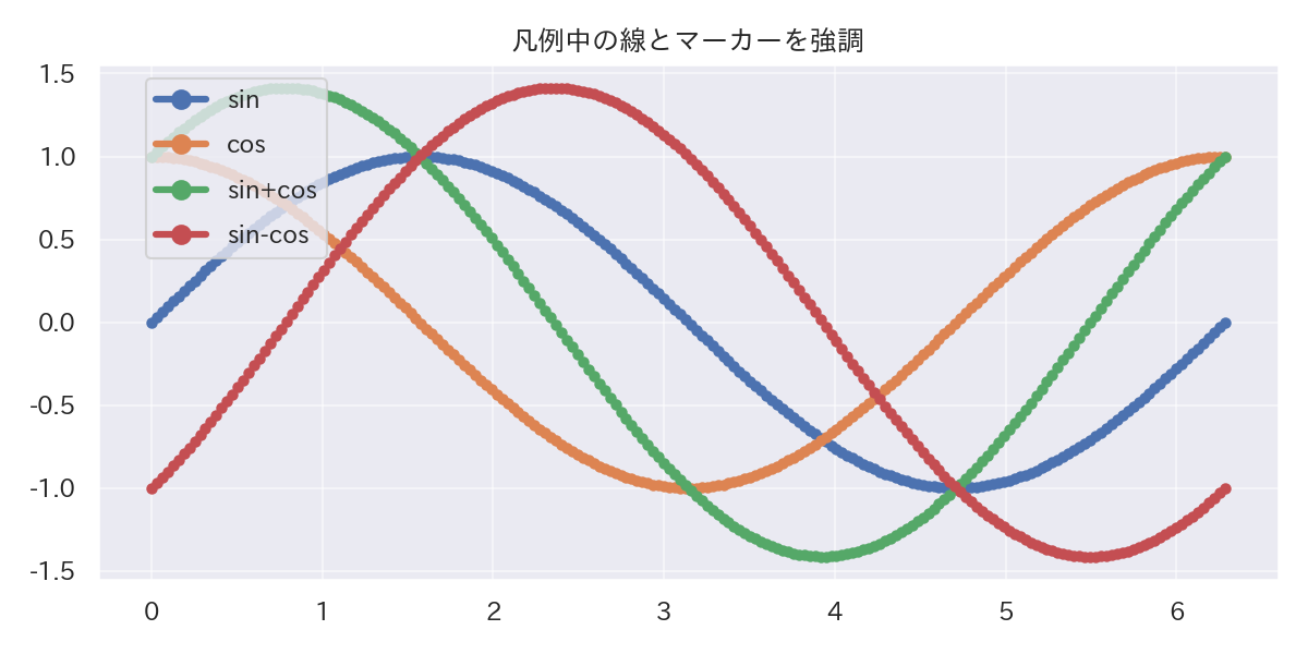
5. 凡例内の線幅・マーカーを強調
#
 1
 2
 3
 4
 5
 6
 7
 8
 9
10
11
12
13
14
15
16
17
| fig, ax = plt.subplots(figsize=(8, 4))
for label, y in series.items():
ax.plot(x, y, marker="o", markersize=4, label=label)
legend = ax.legend(
loc="upper left",
bbox_to_anchor=(0.02, 1.02),
)
handles = getattr(legend, "legendHandles", legend.legend_handles)
for handle in handles:
handle.set_linewidth(3.0)
handle.set_markersize(8)
ax.set_title("凡例中の線とマーカーを強調")
plt.tight_layout()
plt.show()
|
legend.legendHandles(または legend.legend_handles)で Line2D を取得し、凡例だけ線幅やマーカーサイズを太くできます。- プレゼン資料など凡例だけで線種を識別してもらうシーンに有効です。
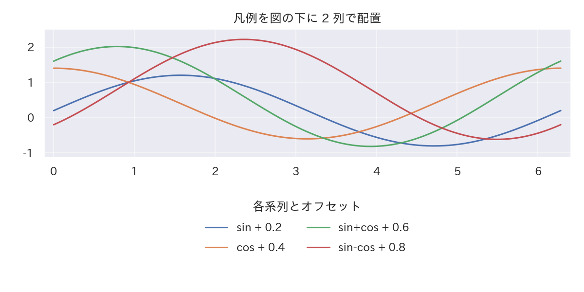
6. 凡例を二段組で図の下に配置
#
 1
 2
 3
 4
 5
 6
 7
 8
 9
10
11
12
13
14
15
| fig, ax = plt.subplots(figsize=(8, 4))
for idx, (label, y) in enumerate(series.items(), start=1):
ax.plot(x, y + idx * 0.2, label=f"{label} + {idx*0.2:.1f}")
ax.legend(
loc="upper center",
bbox_to_anchor=(0.5, -0.22),
ncol=2,
title="各系列とオフセット",
frameon=False,
)
ax.margins(x=0.02, y=0.1)
ax.set_title("凡例を図の下に 2 列で配置")
plt.tight_layout()
plt.show()
|
bbox_to_anchor の y 座標をマイナスにすると、凡例を図の下側に送れます。plt.tight_layout() と組み合わせると凡例がページ外にはみ出しません。
7. 面グラフや基準線の凡例
#
 1
 2
 3
 4
 5
 6
 7
 8
 9
10
11
12
13
14
| fig, ax = plt.subplots(figsize=(8, 4))
ax.fill_between(x, np.sin(x), color="#3b82f6", alpha=0.35, label="元データ範囲")
ax.fill_between(x, np.sin(x), np.sin(x) + 0.3, color="#10b981", alpha=0.45, label="上振れ幅")
ax.axhline(0, color="#475569", linestyle="--", linewidth=1.2, label="基準線")
ax.legend(
loc="upper right",
bbox_to_anchor=(1.02, 1.0),
borderpad=0.8,
)
ax.set_ylim(-1.5, 1.8)
ax.set_title("fill_between + 基準線の凡例")
plt.tight_layout()
plt.show()
|
- 面グラフ(
fill_between)や基準線も凡例に含めると、意味が伝わりやすくなります。 bbox_to_anchor=(1.02, 1.0) で凡例をわずかに右へずらし、面グラフと重ならないようにしています。
いつ使うか
#
- 適している場面: matplotlibの凡例の位置・表示・見た目を自在に調整したいとき。プロットと重ならない配置が学べます。
- 不向きな場面: 凡例が不要なほどシンプルな図(1系列のみなど)にまで凡例を付けると情報過多になります。
- 代替手段: 系列数が少なければ直接ラベル(データ点の近くにテキスト)の方がスッキリ伝わります。
よくある失敗パターン
#
- 凡例がプロット領域と重なる: デフォルト位置の凡例がデータを隠してしまうことがあります。bbox_to_anchor で図の外に配置するか、空白部分に移動してください。
- 凡例の項目が多すぎる: 10 項目以上の凡例は読むのが大変で色の区別も困難です。グルーピングして項目数を減らすか、直接ラベルに切り替えましょう。