Regresión logística | Modelar probabilidades de clase con la sigmoide

Creado: 2019-02-02 Última actualización: 2020-01-29 Tiempo de lectura: 3 min

まとめ

La regresión logística aplica una combinación lineal de las entradas a la función sigmoide para predecir la probabilidad de que la etiqueta sea 1.
La salida está en $[0, 1]$, lo que permite fijar umbrales de decisión con flexibilidad y leer los coeficientes como contribuciones al logit.
El entrenamiento minimiza la entropía cruzada (equivale a maximizar la verosimilitud); la regularización L1/L2 ayuda a evitar el sobreajuste.
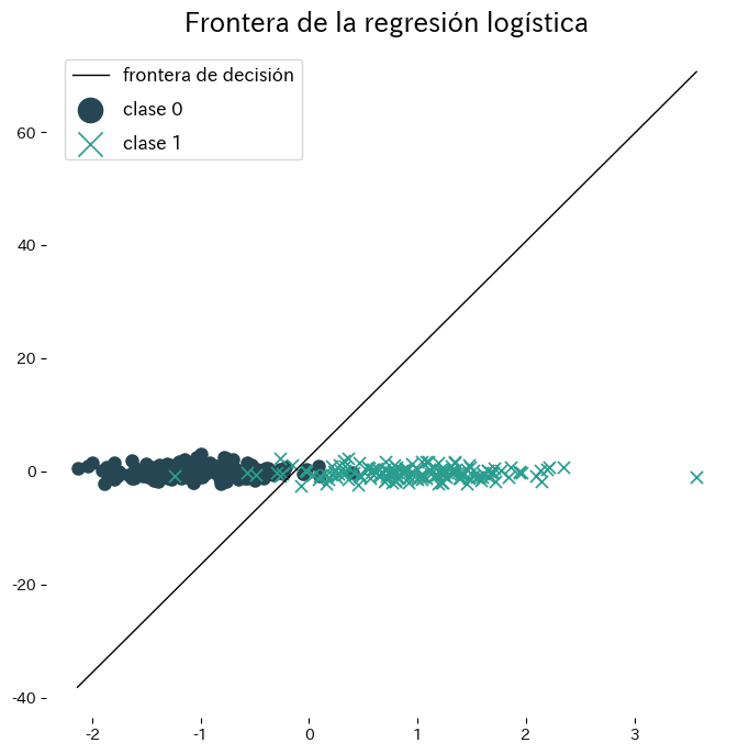
Con LogisticRegression de scikit-learn se cubren el preprocesamiento, el ajuste y la visualización de la frontera de decisión en pocas líneas.

Intuición #

La regresión lineal produce valores reales, pero en clasificación suele interesar “¿cuál es la probabilidad de la clase 1?”. La regresión logística aborda el problema pasando el puntaje lineal $z = \mathbf{w}^\top \mathbf{x} + b$ por la función sigmoide $\sigma(z) = 1 / (1 + e^{-z})$, obteniendo valores con interpretación probabilística. Una regla simple, como “predecir 1 si $P(y=1 \mid \mathbf{x}) > 0.5$”, basta para clasificar.

Formulación matemática #

La probabilidad de la clase 1 dada $\mathbf{x}$ es

$$ P(y=1 \mid \mathbf{x}) = \sigma(\mathbf{w}^\top \mathbf{x} + b) = \frac{1}{1 + \exp\left(-(\mathbf{w}^\top \mathbf{x} + b)\right)}. $$

El aprendizaje maximiza la log-verosimilitud

$$ \ell(\mathbf{w}, b) = \sum_{i=1}^{n} \Bigl[ y_i \log p_i + (1 - y_i) \log (1 - p_i) \Bigr], \quad p_i = \sigma(\mathbf{w}^\top \mathbf{x}_i + b), $$

o, de forma equivalente, minimiza la entropía cruzada negativa. Agregar regularización L2 evita coeficientes inestables, mientras que L1 puede anular características irrelevantes.

Experimentos con Python #

El siguiente ejemplo ajusta la regresión logística a un conjunto sintético bidimensional y visualiza la frontera resultante. Gracias a scikit-learn, entrenar y trazar la frontera requiere pocas líneas.

from __future__ import annotations

import japanize_matplotlib
import matplotlib.pyplot as plt
import numpy as np
from matplotlib.colors import ListedColormap
from sklearn.datasets import make_classification
from sklearn.linear_model import LogisticRegression
from sklearn.metrics import accuracy_score


def run_logistic_regression_demo(
    n_samples: int = 300,
    random_state: int = 2,
    label_class0: str = "clase 0",
    label_class1: str = "clase 1",
    label_boundary: str = "frontera de decisión",
    title: str = "Frontera de la regresión logística",
) -> dict[str, float]:
    """Train logistic regression on a synthetic 2D dataset and visualise the boundary.

    Args:
        n_samples: Number of samples to generate.
        random_state: Seed for reproducible sampling.
        label_class0: Legend label for class 0.
        label_class1: Legend label for class 1.
        label_boundary: Legend label for the separating line.
        title: Title for the plot.

    Returns:
        Dictionary containing training accuracy and coefficients.
    """
    japanize_matplotlib.japanize()
    X, y = make_classification(
        n_samples=n_samples,
        n_features=2,
        n_redundant=0,
        n_informative=2,
        random_state=random_state,
        n_clusters_per_class=1,
    )

    clf = LogisticRegression()
    clf.fit(X, y)

    accuracy = float(accuracy_score(y, clf.predict(X)))
    coef = clf.coef_[0]
    intercept = float(clf.intercept_[0])

    x1, x2 = X[:, 0], X[:, 1]
    grid_x1, grid_x2 = np.meshgrid(
        np.linspace(x1.min() - 1.0, x1.max() + 1.0, 200),
        np.linspace(x2.min() - 1.0, x2.max() + 1.0, 200),
    )
    grid = np.c_[grid_x1.ravel(), grid_x2.ravel()]
    probs = clf.predict_proba(grid)[:, 1].reshape(grid_x1.shape)

    cmap = ListedColormap(["#aec7e8", "#ffbb78"])
    fig, ax = plt.subplots(figsize=(7, 6))
    contour = ax.contourf(grid_x1, grid_x2, probs, levels=20, cmap=cmap, alpha=0.4)
    ax.contour(grid_x1, grid_x2, probs, levels=[0.5], colors="k", linewidths=1.5)
    ax.scatter(x1[y == 0], x2[y == 0], marker="o", edgecolor="k", label=label_class0)
    ax.scatter(x1[y == 1], x2[y == 1], marker="x", color="k", label=label_class1)
    ax.set_xlabel("característica 1")
    ax.set_ylabel("característica 2")
    ax.set_title(title)
    ax.legend(loc="best")
    fig.colorbar(contour, ax=ax, label="P(class = 1)")
    fig.tight_layout()
    plt.show()

    return {
        "accuracy": accuracy,
        "coef_0": float(coef[0]),
        "coef_1": float(coef[1]),
        "intercept": intercept,
    }


metrics = run_logistic_regression_demo(
    label_class0="clase 0",
    label_class1="clase 1",
    label_boundary="frontera de decisión",
    title="Frontera de la regresión logística",
)
print(f"Precisión de entrenamiento: {metrics['accuracy']:.3f}")
print(f"Coeficiente de la característica 1: {metrics['coef_0']:.3f}")
print(f"Coeficiente de la característica 2: {metrics['coef_1']:.3f}")
print(f"Intercepto: {metrics['intercept']:.3f}")

Gracias a scikit-learn, entrenar y trazar la frontera requie… (figura)

Referencias #

Agresti, A. (2015). Foundations of Linear and Generalized Linear Models. Wiley.
Hastie, T., Tibshirani, R., & Friedman, J. (2009). The Elements of Statistical Learning. Springer.